The MODEL Procedure

General Form Models

Subsections:

Supply and Demand Models

The single equation example shown in the preceding section was written in normalized form and specified as an assignment of the regression function to the dependent variable LHUR. However, sometimes it is impossible or inconvenient to write a nonlinear model in normalized form.

To write a general form equation, give the equation a name with the prefix "EQ.". This EQ.-prefixed variable represents the equation error. Write the equation as an assignment to this variable.

For example, suppose you have the following nonlinear model that relates the variables x and y :

${\epsilon } = a + b ~ {\ln }( c y + d x )$

Naming this equation ‘one’, you can fit this model with the following statements:

   proc model data=xydata;
      eq.one = a + b * log( c * y + d * x );
      fit one;
   run;

The use of the EQ. prefix tells PROC MODEL that the variable is an error term and that it should not expect actual values for the variable ONE in the input data set.

Supply and Demand Models

General form specifications are often useful when you have several equations for the same dependent variable. This is common in supply and demand models, where both the supply equation and the demand equation are written as predictions for quantity as functions of price.

For example, consider the following supply and demand system:

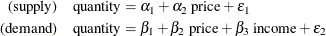
$\begin{align*} \text {(supply)}\quad \text {quantity} & = {\alpha }_{1} + {\alpha }_{2} ~ \text {price} + {\epsilon }_{1} \\ \text {(demand)}\quad \text {quantity} & = {\beta }_{1} + {\beta }_{2} ~ \text {price} + {\beta }_{3} ~ \text {income} + {\epsilon }_{2} \end{align*}$

Assume the quantity of interest is the amount of energy consumed in the U.S., the price is the price of gasoline, and the income variable is the consumer debt. When the market is at equilibrium, these equations determine the market price and the equilibrium quantity. These equations are written in general form as

${\epsilon }_{1} = quantity - ({\alpha }_{1} + {\alpha }_{2} ~ price )$

${\epsilon }_{2} = quantity - ({\beta }_{1} + {\beta }_{2} ~ price + {\beta }_{3} ~ income)$

Note that the endogenous variables quantity and price depend on two error terms so that OLS should not be used. The following example uses three-stage least squares estimation.

Data for this model is obtained from the SASHELP.CITIMON data set.

title1 'Supply-Demand Model using General-form Equations';
proc model data=sashelp.citimon;
   endogenous eegp eec;
   exogenous exvus cciutc;
   parameters a1 a2 b1 b2 b3 ;
   label eegp   = 'Gasoline Retail Price'
         eec    = 'Energy Consumption'
         cciutc = 'Consumer Debt';

   /* -------- Supply equation ------------- */
   eq.supply = eec - (a1 + a2 * eegp);

   /* -------- Demand equation ------------- */
   eq.demand = eec - (b1 + b2 * eegp + b3 * cciutc);

   /* -------- Instrumental variables -------*/
   lageegp = lag(eegp); lag2eegp=lag2(eegp);

   /* -------- Estimate parameters --------- */
   fit supply demand / n3sls fsrsq;
   instruments _EXOG_ lageegp lag2eegp;
run;

The FIT statement specifies the two equations to estimate and the method of estimation, N3SLS. Note that ‘3SLS’ is an alias for N3SLS. The option FSRSQ is selected to get a report of the first stage R $^{2}$ to determine the acceptability of the selected instruments.

Since three-stage least squares is an instrumental variables method, instruments are specified with the INSTRUMENTS statement. The instruments selected are all the exogenous variables, selected with the _EXOG_ option, and two lags of the variable EEGP: LAGEEGP and LAG2EEGP.

The data set CITIMON has four observations that generate missing values because values for EEGP, EEC, or CCIUTC are missing. This is revealed in the "Observations Processed" output shown in Figure 26.7. Missing values are also generated when the equations cannot be computed for a given observation. Missing observations are not used in the estimation.

Figure 26.7: Supply-Demand Observations Processed

Supply-Demand Model using General-form Equations

The MODEL Procedure

3SLS Estimation Summary

Observations Processed
Read	145
Solved	143
First	3
Last	145
Used	139
Missing	4
Lagged	2

The lags used to create the instruments also reduce the number of observations used. In this case, the first two observations were used to fill the lags of EEGP.

The data set has a total of 145 observations, of which four generated missing values and two were used to fill lags, which left 139 observations for the estimation. In the estimation summary, in Figure 26.8, the total degrees of freedom for the model and error is 139.

Figure 26.8: Supply-Demand Parameter Estimates

Supply-Demand Model using General-form Equations

The MODEL Procedure

Nonlinear 3SLS Summary of Residual Errors
Equation	DF Model	DF Error	SSE	MSE	Root MSE	R-Square	Adj R-Sq
supply	2	137	43.2677	0.3158	0.5620
demand	3	136	39.5791	0.2910	0.5395

Nonlinear 3SLS Parameter Estimates
Parameter	Estimate	Approx Std Err	t Value	Approx Pr > \|t\|	1st Stage R-Square
a1	7.30952	0.3799	19.24	<.0001	1.0000
a2	-0.00853	0.00328	-2.60	0.0103	0.9617
b1	6.82196	0.3788	18.01	<.0001	1.0000
b2	-0.00614	0.00303	-2.02	0.0450	0.9617
b3	9E-7	3.165E-7	2.84	0.0051	1.0000

One disadvantage of specifying equations in general form is that there are no actual values associated with the equation, so the R $^{2}$ statistic cannot be computed.