Nonlinear Optimization Methods
The following table summarizes the options available in the NLO system.
Table 6.1: NLO options
|
Option |
Description |
|---|---|
|
Optimization Specifications |
|
|
TECHNIQUE= |
minimization technique |
|
UPDATE= |
update technique |
|
LINESEARCH= |
line-search method |
|
LSPRECISION= |
line-search precision |
|
HESCAL= |
type of Hessian scaling |
|
INHESSIAN= |
start for approximated Hessian |
|
RESTART= |
iteration number for update restart |
|
Termination Criteria Specifications |
|
|
MAXFUNC= |
maximum number of function calls |
|
MAXITER= |
maximum number of iterations |
|
MINITER= |
minimum number of iterations |
|
MAXTIME= |
upper limit seconds of CPU time |
|
ABSCONV= |
absolute function convergence criterion |
|
ABSFCONV= |
absolute function convergence criterion |
|
ABSGCONV= |
absolute gradient convergence criterion |
|
ABSXCONV= |
absolute parameter convergence criterion |
|
FCONV= |
relative function convergence criterion |
|
FCONV2= |
relative function convergence criterion |
|
GCONV= |
relative gradient convergence criterion |
|
XCONV= |
relative parameter convergence criterion |
|
FSIZE= |
used in FCONV, GCONV criterion |
|
XSIZE= |
used in XCONV criterion |
|
Step Length Options |
|
|
DAMPSTEP= |
damped steps in line search |
|
MAXSTEP= |
maximum trust region radius |
|
INSTEP= |
initial trust region radius |
|
Printed Output Options |
|
|
PALL |
display (almost) all printed optimization-related output |
|
PHISTORY |
display optimization history |
|
PHISTPARMS |
display parameter estimates in each iteration |
|
PSHORT |
reduce some default optimization-related output |
|
PSUMMARY |
reduce most default optimization-related output |
|
NOPRINT |
suppress all printed optimization-related output |
|
Remote Monitoring Options |
|
|
SOCKET= |
specify the fileref for remote monitoring |
These options are described in alphabetical order.
-
ABSCONV=r
ABSTOL=r -
specifies an absolute function convergence criterion. For minimization, termination requires
 . The default value of r is the negative square root of the largest double-precision value, which serves only as a protection against overflows.
-
ABSFCONV=
![$r[n]$](images/etsug_nlomet0002.png)
ABSFTOL=
-
specifies an absolute function convergence criterion. For all techniques except NMSIMP, termination requires a small change of the function value in successive iterations:
![\[ |f(\theta ^{(k-1)}) - f(\theta ^{(k)})| \leq r \]](images/etsug_nlomet0003.png)
The same formula is used for the NMSIMP technique, but
 is defined as the vertex with the lowest function value, and
  is defined as the vertex with the highest function value in the simplex. The default value is
  . The optional integer value n specifies the number of successive iterations for which the criterion must be satisfied before the process can be terminated.
-
ABSGCONV=
ABSGTOL=
-
specifies an absolute gradient convergence criterion. Termination requires the maximum absolute gradient element to be small:
![\[ \max _ j |g_ j(\theta ^{(k)})| \leq r \]](images/etsug_nlomet0007.png)
This criterion is not used by the NMSIMP technique. The default value is
 . The optional integer value n specifies the number of successive iterations for which the criterion must be satisfied before the process can be terminated.
-
ABSXCONV=
ABSXTOL=
-
specifies an absolute parameter convergence criterion. For all techniques except NMSIMP, termination requires a small Euclidean distance between successive parameter vectors,
![\[ \parallel \theta ^{(k)} - \theta ^{(k-1)} \parallel _2 \leq r \]](images/etsug_nlomet0009.png)
For the NMSIMP technique, termination requires either a small length
 of the vertices of a restart simplex,
![\[ \alpha ^{(k)} \leq r \]](images/etsug_nlomet0011.png)
or a small simplex size,
![\[ \delta ^{(k)} \leq r \]](images/etsug_nlomet0012.png)
where the simplex size
 is defined as the L1 distance from the simplex vertex
  with the smallest function value to the other n simplex points
  :
:
![\[ \delta ^{(k)} = \sum _{\theta _ l \neq y} \parallel \theta _ l^{(k)} - \xi ^{(k)}\parallel _1 \]](images/etsug_nlomet0016.png)
The default is
 for the NMSIMP technique and otherwise. The optional integer value n specifies the number of successive iterations for which the criterion must be satisfied before the process can terminate.
- DAMPSTEP[=r]
-
specifies that the initial step length value
 for each line search (used by the QUANEW, HYQUAN, CONGRA, or NEWRAP technique) cannot be larger than r times the step length value used in the former iteration. If the DAMPSTEP option is specified but r is not specified, the default is
  . The DAMPSTEP=r option can prevent the line-search algorithm from repeatedly stepping into regions where some objective functions are difficult
to compute or where they could lead to floating point overflows during the computation of objective functions and their derivatives.
The DAMPSTEP=r option can save time-costly function calls during the line searches of objective functions that result in very small steps.
. The DAMPSTEP=r option can prevent the line-search algorithm from repeatedly stepping into regions where some objective functions are difficult
to compute or where they could lead to floating point overflows during the computation of objective functions and their derivatives.
The DAMPSTEP=r option can save time-costly function calls during the line searches of objective functions that result in very small steps.
-
FCONV=
FTOL=
-
specifies a relative function convergence criterion. For all techniques except NMSIMP, termination requires a small relative change of the function value in successive iterations,
![\[ { \frac{ |f(\theta ^{(k)}) - f(\theta ^{(k-1)})|}{\max (|f(\theta ^{(k-1)})|,\mbox{FSIZE})} } \leq r \]](images/etsug_nlomet0020.png)
where FSIZE is defined by the FSIZE= option. The same formula is used for the NMSIMP technique, but
is defined as the vertex with the lowest function value, and is defined as the vertex with the highest function value in the simplex. The default value may depend on the procedure. In
most cases, you can use the PALL option to find it.
-
FCONV2=
FTOL2=
-
specifies another function convergence criterion.
For all techniques except NMSIMP, termination requires a small predicted reduction
![\[ df^{(k)} \approx f(\theta ^{(k)}) - f(\theta ^{(k)} + s^{(k)}) \]](images/etsug_nlomet0021.png)
of the objective function. The predicted reduction
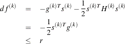
is computed by approximating the objective function f by the first two terms of the Taylor series and substituting the Newton step
![\[ s^{(k)} = - [H^{(k)}]^{-1} g^{(k)} \]](images/etsug_nlomet0023.png)
For the NMSIMP technique, termination requires a small standard deviation of the function values of the
 simplex vertices
  ,
,  ,
, ![$ \sqrt { \frac{1}{n+1} \sum _ l \left[ f(\theta _ l^{(k)}) - \overline{f}(\theta ^{(k)}) \right]^2 } \leq r $](images/etsug_nlomet0027.png) where
where 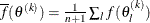 . If there are
  boundary constraints active at , the mean and standard deviation are computed only for the
  unconstrained vertices.
The default value is
 for the NMSIMP technique and otherwise. The optional integer value n specifies the number of successive iterations for which the criterion must be satisfied before the process can terminate.
- FSIZE=r
-
specifies the FSIZE parameter of the relative function and relative gradient termination criteria. The default value is
. For more details, see the FCONV= and GCONV= options.
-
GCONV=
GTOL=
-
specifies a relative gradient convergence criterion. For all techniques except CONGRA and NMSIMP, termination requires that the normalized predicted function reduction is small,
![\[ frac{ g(\theta ^{(k)})^ T [H^{(k)}]^{-1} g(\theta ^{(k)})} {\max (|f(\theta ^{(k)})|,\mbox{FSIZE}) } \leq r \]](images/etsug_nlomet0032.png)
where FSIZE is defined by the FSIZE= option. For the CONGRA technique (where a reliable Hessian estimate
 is not available), the following criterion is used:
![\[ \frac{ \parallel g(\theta ^{(k)}) \parallel _2^2 \quad \parallel s(\theta ^{(k)}) \parallel _2}{\parallel g(\theta ^{(k)}) - g(\theta ^{(k-1)}) \parallel _2 \max (|f(\theta ^{(k)})|,\mbox{FSIZE}) } \leq r \]](images/etsug_nlomet0034.png)
This criterion is not used by the NMSIMP technique. The default value is
 . The optional integer value n specifies the number of successive iterations for which the criterion must be satisfied before the process can terminate.
-
HESCAL=

HS=
-
specifies the scaling version of the Hessian matrix used in NRRIDG, TRUREG, NEWRAP, or DBLDOG optimization.
If HS is not equal to 0, the first iteration and each restart iteration sets the diagonal scaling matrix
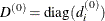 :
:
![\[ d_ i^{(0)} = \sqrt {\max (|H^{(0)}_{i,i}|,\epsilon )} \]](images/etsug_nlomet0038.png)
where
 are the diagonal elements of the Hessian. In every other iteration, the diagonal scaling matrix is updated depending on the HS option:
In each scaling update,
 is the relative machine precision. The default value is HS=0. Scaling of the Hessian can be time consuming in the case where
general linear constraints are active.
is the relative machine precision. The default value is HS=0. Scaling of the Hessian can be time consuming in the case where
general linear constraints are active.
-
INHESSIAN[= r ]
INHESS[= r ] -
specifies how the initial estimate of the approximate Hessian is defined for the quasi-Newton techniques QUANEW and DBLDOG. There are two alternatives:
-
If you do not use the r specification, the initial estimate of the approximate Hessian is set to the Hessian at
 .
.
-
If you do use the r specification, the initial estimate of the approximate Hessian is set to the multiple of the identity matrix
 .
.
By default, if you do not specify the option INHESSIAN=r, the initial estimate of the approximate Hessian is set to the multiple of the identity matrix
, where the scalar r is computed from the magnitude of the initial gradient.
-
- INSTEP=r
-
reduces the length of the first trial step during the line search of the first iterations. For highly nonlinear objective functions, such as the EXP function, the default initial radius of the trust-region algorithm TRUREG or DBLDOG or the default step length of the line-search algorithms can result in arithmetic overflows. If this occurs, you should specify decreasing values of
 such as INSTEP=
 , INSTEP=
 , INSTEP=
 , and so on, until the iteration starts successfully.
-
For trust-region algorithms (TRUREG, DBLDOG), the INSTEP= option specifies a factor
 for the initial radius
  of the trust region. The default initial trust-region radius is the length of the scaled gradient. This step corresponds
to the default radius factor of
of the trust region. The default initial trust-region radius is the length of the scaled gradient. This step corresponds
to the default radius factor of  .
.
-
For line-search algorithms (NEWRAP, CONGRA, QUANEW), the INSTEP= option specifies an upper bound for the initial step length for the line search during the first five iterations. The default initial step length is
.
-
For the Nelder-Mead simplex algorithm, using TECH=NMSIMP, the INSTEP=r option defines the size of the start simplex.
-
-
LINESEARCH=i
LIS=i -
specifies the line-search method for the CONGRA, QUANEW, and NEWRAP optimization techniques. See Fletcher (1987) for an introduction to line-search techniques. The value of i can be
 . For CONGRA, QUANEW and NEWRAP, the default value is
  .
.
- LIS=1
-
specifies a line-search method that needs the same number of function and gradient calls for cubic interpolation and cubic extrapolation; this method is similar to one used by the Harwell subroutine library.
- LIS=2
-
specifies a line-search method that needs more function than gradient calls for quadratic and cubic interpolation and cubic extrapolation; this method is implemented as shown in Fletcher (1987) and can be modified to an exact line search by using the LSPRECISION= option.
- LIS=3
-
specifies a line-search method that needs the same number of function and gradient calls for cubic interpolation and cubic extrapolation; this method is implemented as shown in Fletcher (1987) and can be modified to an exact line search by using the LSPRECISION= option.
- LIS=4
-
specifies a line-search method that needs the same number of function and gradient calls for stepwise extrapolation and cubic interpolation.
- LIS=5
-
specifies a line-search method that is a modified version of LIS=4.
- LIS=6
-
specifies golden section line search (Polak, 1971), which uses only function values for linear approximation.
- LIS=7
-
specifies bisection line search (Polak, 1971), which uses only function values for linear approximation.
- LIS=8
-
specifies the Armijo line-search technique (Polak, 1971), which uses only function values for linear approximation.
-
LSPRECISION=r
LSP=r -
specifies the degree of accuracy that should be obtained by the line-search algorithms LIS=2 and LIS=3. Usually an imprecise line search is inexpensive and successful. For more difficult optimization problems, a more precise and expensive line search may be necessary (Fletcher, 1987). The second line-search method (which is the default for the NEWRAP, QUANEW, and CONGRA techniques) and the third line-search method approach exact line search for small LSPRECISION= values. If you have numerical problems, you should try to decrease the LSPRECISION= value to obtain a more precise line search. The default values are shown in the following table.
Table 6.2: Line Search Precision Defaults
TECH=
UPDATE=
LSP default
QUANEW
DBFGS, BFGS
r = 0.4
QUANEW
DDFP, DFP
r = 0.06
CONGRA
all
r = 0.1
NEWRAP
no update
r = 0.9
For more details, see Fletcher (1987).
-
MAXFUNC=i
MAXFU=i -
specifies the maximum number i of function calls in the optimization process. The default values are
-
TRUREG, NRRIDG, NEWRAP: 125
-
QUANEW, DBLDOG: 500
-
CONGRA: 1000
-
NMSIMP: 3000
Note that the optimization can terminate only after completing a full iteration. Therefore, the number of function calls that is actually performed can exceed the number that is specified by the MAXFUNC= option.
-
-
MAXITER=i
MAXIT=i -
specifies the maximum number i of iterations in the optimization process. The default values are
-
TRUREG, NRRIDG, NEWRAP: 50
-
QUANEW, DBLDOG: 200
-
CONGRA: 400
-
NMSIMP: 1000
These default values are also valid when i is specified as a missing value.
-
-
MAXSTEP=
-
specifies an upper bound for the step length of the line-search algorithms during the first n iterations. By default, r is the largest double-precision value and n is the largest integer available. Setting this option can improve the speed of convergence for the CONGRA, QUANEW, and NEWRAP techniques.
- MAXTIME=r
-
specifies an upper limit of r seconds of CPU time for the optimization process. The default value is the largest floating-point double representation of your computer. Note that the time specified by the MAXTIME= option is checked only once at the end of each iteration. Therefore, the actual running time can be much longer than that specified by the MAXTIME= option. The actual running time includes the rest of the time needed to finish the iteration and the time needed to generate the output of the results.
-
MINITER=i
MINIT=i -
specifies the minimum number of iterations. The default value is 0. If you request more iterations than are actually needed for convergence to a stationary point, the optimization algorithms can behave strangely. For example, the effect of rounding errors can prevent the algorithm from continuing for the required number of iterations.
- NOPRINT
-
suppresses the output. (See procedure documentation for availability of this option.)
- PALL
-
displays all optional output for optimization. (See procedure documentation for availability of this option.)
- PHISTORY
-
displays the optimization history. (See procedure documentation for availability of this option.)
- PHISTPARMS
-
display parameter estimates in each iteration. (See procedure documentation for availability of this option.)
- PINIT
-
displays the initial values and derivatives (if available). (See procedure documentation for availability of this option.)
- PSHORT
-
restricts the amount of default output. (See procedure documentation for availability of this option.)
- PSUMMARY
-
restricts the amount of default displayed output to a short form of iteration history and notes, warnings, and errors. (See procedure documentation for availability of this option.)
-
RESTART=

REST=
-
specifies that the QUANEW or CONGRA algorithm is restarted with a steepest descent/ascent search direction after, at most, i iterations. Default values are as follows:
-
CONGRA UPDATE=PB: restart is performed automatically, i is not used.
-
CONGRA UPDATE
 PB:
PB:  , where n is the number of parameters.
-
QUANEW i is the largest integer available.
-
- SOCKET=fileref
-
Specifies the fileref that contains the information needed for remote monitoring. See the section Remote Monitoring for more details.
-
TECHNIQUE=value
TECH=value -
specifies the optimization technique. Valid values are as follows:
-
CONGRA performs a conjugate-gradient optimization, which can be more precisely specified with the UPDATE= option and modified with the LINESEARCH= option. When you specify this option, UPDATE=PB by default.
-
DBLDOG performs a version of double-dogleg optimization, which can be more precisely specified with the UPDATE= option. When you specify this option, UPDATE=DBFGS by default.
-
NMSIMP performs a Nelder-Mead simplex optimization.
-
NONE does not perform any optimization. This option can be used as follows:
-
to perform a grid search without optimization
-
to compute estimates and predictions that cannot be obtained efficiently with any of the optimization techniques
-
-
NEWRAP performs a Newton-Raphson optimization that combines a line-search algorithm with ridging. The line-search algorithm LIS=2 is the default method.
-
NRRIDG performs a Newton-Raphson optimization with ridging.
-
QUANEW performs a quasi-Newton optimization, which can be defined more precisely with the UPDATE= option and modified with the LINESEARCH= option. This is the default estimation method.
-
TRUREG performs a trust region optimization.
-
-
UPDATE=method
UPD=method -
specifies the update method for the QUANEW, DBLDOG, or CONGRA optimization technique. Not every update method can be used with each optimizer.
Valid methods are as follows:
-
BFGS performs the original Broyden, Fletcher, Goldfarb, and Shanno (BFGS) update of the inverse Hessian matrix.
-
DBFGS performs the dual BFGS update of the Cholesky factor of the Hessian matrix. This is the default update method.
-
DDFP performs the dual Davidon, Fletcher, and Powell (DFP) update of the Cholesky factor of the Hessian matrix.
-
DFP performs the original DFP update of the inverse Hessian matrix.
-
PB performs the automatic restart update method of Powell (1977); Beale (1972).
-
FR performs the Fletcher-Reeves update (Fletcher, 1987).
-
PR performs the Polak-Ribiere update (Fletcher, 1987).
-
CD performs a conjugate-descent update of Fletcher (1987).
-
-
XCONV=
XTOL=
-
specifies the relative parameter convergence criterion. For all techniques except NMSIMP, termination requires a small relative parameter change in subsequent iterations.
![\[ \frac{\max _ j |\theta _ j^{(k)} - \theta _ j^{(k-1)}|}{\max (|\theta _ j^{(k)}|,|\theta _ j^{(k-1)}|,\mbox{XSIZE})} \leq r \]](images/etsug_nlomet0059.png)
For the NMSIMP technique, the same formula is used, but
 is defined as the vertex with the lowest function value and
  is defined as the vertex with the highest function value in the simplex. The default value is for the NMSIMP technique and otherwise. The optional integer value n specifies the number of successive iterations for which the criterion must be satisfied before the process can be terminated.
-
XSIZE=

-
specifies the XSIZE parameter of the relative parameter termination criterion. The default value is
. For more detail, see the XCONV= option.