The MODEL Procedure
PROC MODEL provides several features to aid in analyzing the structure of the model program. These features summarize properties of the model in various forms.
During the development of model programs for simulation, misspecification of the equations or variables that compose the systems of nonlinear equations is common. These misspecification errors can occur both in the original formulation of the model and in the encoding of the model into PROC MODEL statements. For large systems these errors can be difficult and time consuming to isolate and repair. Similarly, the process of becoming familiar with an existing simulation model that is encoded in PROC MODEL can be laborious when available documentation is insufficient to understand the model’s implementation. To address these issues, the ANALYZEDEP= option can be applied to SOLVE steps to produce graphical analyses of a model’s structure.
The graphical output that is produced by the ANALYZEDEP= option displays the results of two separate, hierarchical analyses that are both based on the dependence of equations on solve variables in the nonlinear system of equations. First, the system is partitioned to identify which equations overdetermine solve variables, which equations underdetermine solve variables, and which equations consistently determine solve variables. These three partitions of equations and their corresponding three partitions of solve variables are identified in the graphical output and listing produced by the ANALYZEDEP= option. Second, each partition from the first analysis is analyzed to identify subpartitions of equations and solve variables such that all the solve variables within each subpartition depend either directly or indirectly on one another. In the graphical output the subpartitions are represented as blocks in a dependency matrix. The subpartition blocks are ordered so that the matrix of dependencies has a block upper-triangular form.
The first-level partitioning of the system into underdetermined, overdetermined, and consistent systems of equations and variables uses a Dulmage-Mendelsohn (DM) decomposition to define the three partitions, following the work by Dulmage and Mendelsohn (1958); Pothen and Fan (1990). The overdetermining equations in a DM decomposition are the set of all equations that do not have dependent variables on the diagonal of any dependency matrix that contains the maximum possible number of entries on the diagonal. The dependency matrices for a problem consist of the set of pairs of orderings of the problem’s equations and solve variables. Correspondingly, the DM decomposition defines underdetermined variables as the set of all variables that do not appear on the diagonal of any dependency matrix that contains the maximum number of entries on the diagonal. Therefore, the DM decomposition is canonical in the sense that its partitioning of the system is invariant to the order equations and variables are specified in the model program. The following PROC MODEL statements illustrate how to partition a simple model with five equations and five unknowns:
proc model data=_null_;
   endo a b c d e;

   f(a)     = 0;
   g(a,b)   = 0;
   h(a,b)   = 0;
   i(b,d)   = 0;
   j(c,d,e) = 0;

   solve / analyzedep=(block);
quit;
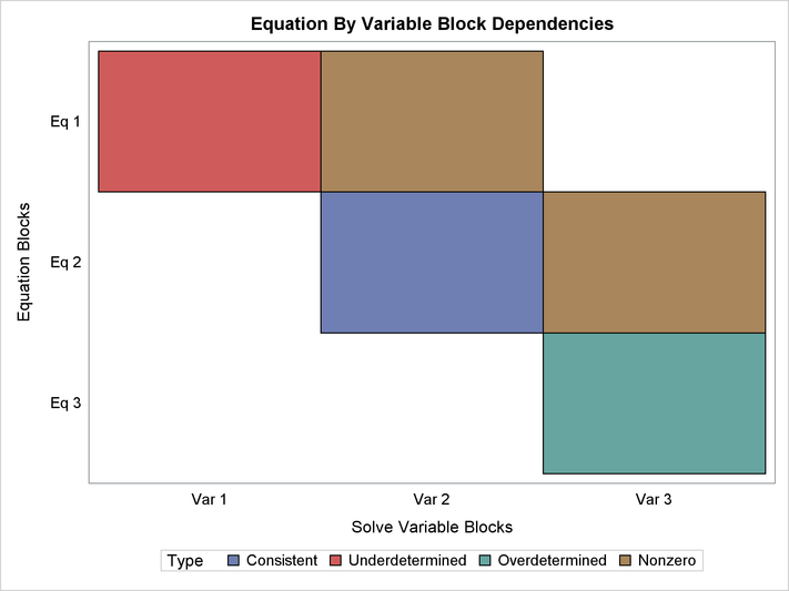
Figure 19.92 and Figure 19.93 illustrate which equations and variables belong to each block and which blocks are in each partition. The cells that are marked “Nonzero” in the plot represent a dependency between blocks that are above the diagonal in the dependency matrix. The exact functional forms of the equations in this example are not shown; however, the dependency analysis here reveals that this model is structurally singular because it contains overdetermined and underdetermined components. Some modification of the model specification is necessary before a SOLVE step can be executed.
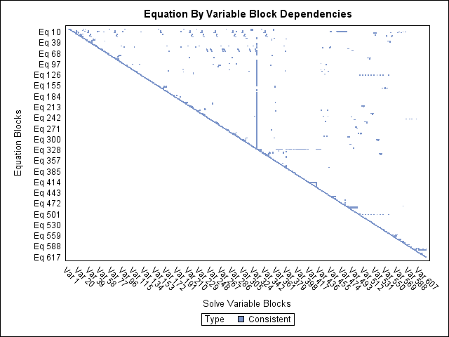
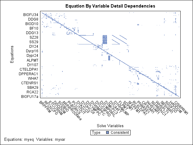
For large systems of equations, the graphical output that the ANALYZEDEP= option produces can be used as a starting point to explore dependency relationships when the models’ programming statement listings and dependency tables are too long to read and comprehend. For example, one econometric model of U.S. agriculture involves thousand of equation and variable dependencies whose structure is difficult to interpret in textual listings of the model. If you examine the block triangular form of its dependency matrix in Figure 19.94, one pattern of dependencies that becomes apparent is the vertical grouping of block dependencies in the middle of the plot. Figure 19.95 shows the dependency matrix for this important subpartition of equations and variables responsible for coupling the vertical grouping of blocks.
Compared to the BLOCK and GRAPH options, the ANALYZEDEP= option has the following advantages:
-
shows which equations and solve variables are overdetermined, consistent, and underdetermined
-
works with any combination of normal form and general form equations
-
can display dependency matrices involving many more equations and variables
-
can be limited to a subset of the equations and variables in the model
The following Klein’s model program is used to introduce the LISTDEP, BLOCK, and GRAPH options:
proc model  out=m data=klein listdep graph block;
   endogenous c p w i x wsum k y;
   exogenous  wp g t year;
   parms c0-c3 i0-i3 w0-w3;
   a: c = c0 + c1 * p + c2 * lag(p) + c3 * wsum;
   b: i = i0 + i1 * p + i2 * lag(p) + i3 * lag(k);
   c: w = w0 + w1 * x + w2 * lag(x) + w3 * year;
   x = c + i + g;
   y = c + i + g-t;
   p = x-w-t;
   k = lag(k) + i;
   wsum = w + wp;
   id year;
quit;
The LISTDEP option produces a dependency list for each variable in the model program. For each variable, a list of variables that depend on it and a list of variables it depends on is given. The dependency list produced by the example program is shown in Figure 19.96.
Figure 19.96: A Portion of the LISTDEP Output for Klein’s Model
| Dependency Listing For Program | |
|---|---|
| Symbol----------- | Dependencies |
| c | Current values affect: RESID.c ERROR.c PRED.x RESID.x ERROR.x PRED.y RESID.y ERROR.y |
| p | Current values affect: PRED.c RESID.c ERROR.c PRED.i RESID.i ERROR.i RESID.p ERROR.p |
| Lagged values affect: PRED.c PRED.i | |
| w | Current values affect: RESID.w ERROR.w PRED.p RESID.p ERROR.p PRED.wsum RESID.wsum ERROR.wsum |
| i | Current values affect: RESID.i ERROR.i PRED.x RESID.x ERROR.x PRED.y RESID.y ERROR.y PRED.k RESID.k ERROR.k |
| x | Current values affect: PRED.w RESID.w ERROR.w RESID.x ERROR.x PRED.p RESID.p ERROR.p |
| Lagged values affect: PRED.w | |
| wsum | Current values affect: PRED.c RESID.c ERROR.c RESID.wsum ERROR.wsum |
| k | Current values affect: RESID.k ERROR.k |
| Lagged values affect: PRED.i RESID.i ERROR.i PRED.k | |
| y | Current values affect: RESID.y ERROR.y |
| wp | Current values affect: PRED.wsum RESID.wsum ERROR.wsum |
| g | Current values affect: PRED.x RESID.x ERROR.x PRED.y RESID.y ERROR.y |
| t | Current values affect: PRED.y RESID.y ERROR.y PRED.p RESID.p ERROR.p |
| year | Current values affect: PRED.w RESID.w ERROR.w |
| c0 | Current values affect: PRED.c RESID.c ERROR.c |
| c1 | Current values affect: PRED.c RESID.c ERROR.c |
| c2 | Current values affect: PRED.c RESID.c ERROR.c |
| c3 | Current values affect: PRED.c RESID.c ERROR.c |
| i0 | Current values affect: PRED.i RESID.i ERROR.i |
| i1 | Current values affect: PRED.i RESID.i ERROR.i |
| i2 | Current values affect: PRED.i RESID.i ERROR.i |
| i3 | Current values affect: PRED.i RESID.i ERROR.i |
| w0 | Current values affect: PRED.w RESID.w ERROR.w |
| w1 | Current values affect: PRED.w RESID.w ERROR.w |
| w2 | Current values affect: PRED.w RESID.w ERROR.w |
| w3 | Current values affect: PRED.w RESID.w ERROR.w |
| PRED.c | Depends on current values of: p wsum c0 c1 c2 c3 |
| Depends on lagged values of: p | |
| Current values affect: RESID.c ERROR.c | |
| RESID.c | Depends on current values of: PRED.c c p wsum c0 c1 c2 c3 |
| ERROR.c | Depends on current values of: PRED.c c p wsum c0 c1 c2 c3 |
| ACTUAL.c | Current values affect: RESID.c ERROR.c PRED.x RESID.x ERROR.x PRED.y RESID.y ERROR.y |
| PRED.i | Depends on current values of: p i0 i1 i2 i3 |
| Depends on lagged values of: p k | |
| Current values affect: RESID.i ERROR.i | |
| RESID.i | Depends on current values of: PRED.i p i i0 i1 i2 i3 |
| Depends on lagged values of: k | |
| ERROR.i | Depends on current values of: PRED.i p i i0 i1 i2 i3 |
| Depends on lagged values of: k | |
| ACTUAL.i | Current values affect: RESID.i ERROR.i PRED.x RESID.x ERROR.x PRED.y RESID.y ERROR.y PRED.k RESID.k ERROR.k |
| PRED.w | Depends on current values of: x year w0 w1 w2 w3 |
| Depends on lagged values of: x | |
| Current values affect: RESID.w ERROR.w | |
| RESID.w | Depends on current values of: PRED.w w x year w0 w1 w2 w3 |
| ERROR.w | Depends on current values of: PRED.w w x year w0 w1 w2 w3 |
| ACTUAL.w | Current values affect: RESID.w ERROR.w PRED.p RESID.p ERROR.p PRED.wsum RESID.wsum ERROR.wsum |
| PRED.x | Depends on current values of: c i g |
| Current values affect: RESID.x ERROR.x | |
| RESID.x | Depends on current values of: PRED.x c i x g |
| ERROR.x | Depends on current values of: PRED.x c i x g |
| ACTUAL.x | Current values affect: PRED.w RESID.w ERROR.w RESID.x ERROR.x PRED.p RESID.p ERROR.p |
| Lagged values affect: PRED.w | |
| PRED.y | Depends on current values of: c i g t |
| Current values affect: RESID.y ERROR.y | |
| RESID.y | Depends on current values of: PRED.y c i y g t |
| ERROR.y | Depends on current values of: PRED.y c i y g t |
| ACTUAL.y | Current values affect: RESID.y ERROR.y |
| PRED.p | Depends on current values of: w x t |
| Current values affect: RESID.p ERROR.p | |
| RESID.p | Depends on current values of: PRED.p p w x t |
| ERROR.p | Depends on current values of: PRED.p p w x t |
| ACTUAL.p | Current values affect: PRED.c RESID.c ERROR.c PRED.i RESID.i ERROR.i RESID.p ERROR.p |
| Lagged values affect: PRED.c PRED.i | |
| PRED.k | Depends on current values of: i |
| Depends on lagged values of: k | |
| Current values affect: RESID.k ERROR.k | |
| RESID.k | Depends on current values of: PRED.k i k |
| ERROR.k | Depends on current values of: PRED.k i k |
| ACTUAL.k | Current values affect: RESID.k ERROR.k |
| Lagged values affect: PRED.i RESID.i ERROR.i PRED.k | |
| PRED.wsum | Depends on current values of: w wp |
| Current values affect: RESID.wsum ERROR.wsum | |
| RESID.wsum | Depends on current values of: PRED.wsum w wsum wp |
| ERROR.wsum | Depends on current values of: PRED.wsum w wsum wp |
| ACTUAL.wsum | Current values affect: PRED.c RESID.c ERROR.c RESID.wsum ERROR.wsum |
The BLOCK option prints an analysis of the program variables based on the assignments in the model program. The output produced by the example is shown in Figure 19.97.
One use for the block output is to put a model in recursive form. Simulations of the model can be done with the SEIDEL method, which is efficient if the model is recursive and if the equations are in recursive order. By examining the block output, you can determine how to reorder the model equations for the most efficient simulation.
The GRAPH option displays the same information as the BLOCK option with the addition of an adjacency graph. An X in a column in an adjacency graph indicates that the variable associated with the row depends on the variable associated with the column. The output produced by the example is shown in Figure 19.98.
The first and last graphs are straightforward. The middle graph represents the dependencies of the nonexogenous variables after transitive closure has been performed (that is, A depends on B, and B depends on C, so A depends on C). The preceding transitive closure matrix indicates that K and Y do not directly or indirectly depend on each other.
Figure 19.98: The GRAPH Output for Klein’s Model
| Adjacency Matrix for Graph of System | |||||||||||||
|---|---|---|---|---|---|---|---|---|---|---|---|---|---|
| Variable | c | p | w | i | x | wsum | k | y | wp | g | t | year | |
| * | * | * | * | ||||||||||
| c | X | X | . | . | . | X | . | . | . | . | . | . | |
| p | . | X | X | . | X | . | . | . | . | . | X | . | |
| w | . | . | X | . | X | . | . | . | . | . | . | X | |
| i | . | X | . | X | . | . | . | . | . | . | . | . | |
| x | X | . | . | X | X | . | . | . | . | X | . | . | |
| wsum | . | . | X | . | . | X | . | . | X | . | . | . | |
| k | . | . | . | X | . | . | X | . | . | . | . | . | |
| y | X | . | . | X | . | . | . | X | . | X | X | . | |
| wp | * | . | . | . | . | . | . | . | . | X | . | . | . |
| g | * | . | . | . | . | . | . | . | . | . | X | . | . |
| t | * | . | . | . | . | . | . | . | . | . | . | X | . |
| year | * | . | . | . | . | . | . | . | . | . | . | . | X |
| (Note: * = Exogenous Variable.) |
| Adjacency Matrix for Graph of System Including Lagged Impacts | ||||||||||||||
|---|---|---|---|---|---|---|---|---|---|---|---|---|---|---|
| Block | Variable | c | p | w | i | x | wsum | k | y | wp | g | t | year | |
| * | * | * | * | |||||||||||
| 1 | c | X | L | . | . | . | X | . | . | . | . | . | . | |
| 1 | p | . | X | X | . | X | . | . | . | . | . | X | . | |
| 1 | w | . | . | X | . | L | . | . | . | . | . | . | X | |
| 1 | i | . | L | . | X | . | . | L | . | . | . | . | . | |
| 1 | x | X | . | . | X | X | . | . | . | . | X | . | . | |
| 1 | wsum | . | . | X | . | . | X | . | . | X | . | . | . | |
| k | . | . | . | X | . | . | L | . | . | . | . | . | ||
| y | X | . | . | X | . | . | . | X | . | X | X | . | ||
| wp | * | . | . | . | . | . | . | . | . | X | . | . | . | |
| g | * | . | . | . | . | . | . | . | . | . | X | . | . | |
| t | * | . | . | . | . | . | . | . | . | . | . | X | . | |
| year | * | . | . | . | . | . | . | . | . | . | . | . | X | |
| (Note: * = Exogenous Variable.) |