The MODEL Procedure
Ordinary differential equations (ODEs) are also called initial value problems because a time zero value for each first-order differential equation is needed. The following is an example of a first-order system of ODEs:
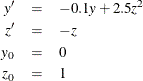
Note that you must provide an initial value for each ODE.
As a reminder, any n-order differential equation can be modeled as a system of first-order differential equations. For example, consider the differential equations
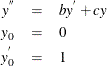
which can be written as the system of differential equations
This differential system can be simulated as follows:
data t;
   time=0; output;
   time=1; output;
   time=2; output;
run;

proc model data=t ;
   dependent y 0 z 1;
   parm b -2 c -4;

   dert.y = z;
   dert.z = b * dert.y + c * y;

   solve y z / dynamic solveprint;
run;
The preceding statements produce the output shown in Figure 19.46. These statements produce additional output, which is not shown.
The differential variables are distinguished by the derivative with respect to time (DERT.) prefix. Once you define the DERT. variable, you can use it on the right-hand side of another equation. The differential equations must be expressed in normal form; implicit differential equations are not allowed, and other terms on the left-hand side are not allowed.
The TIME variable is the implied with respect to variable for all DERT. variables. The TIME variable is also the only variable that must be in the input data set.
You can provide initial values for the differential equations in the data set, in the declaration statement (as in the previous example), or in statements in the program. Using the previous example, you can specify the initial values as
   proc model data=t ;
      dependent y z ;
      parm b -2 c -4;

      if ( time=0 ) then
         do;
            y=0;
            z=1;
         end;
      else
         do;
            dert.y = z;
            dert.z = b * dert.y + c * y;
         end;
      end;

      solve y z / dynamic solveprint;
   run;
If you do not provide an initial value, 0 is used.
Note that, in the previous example, the DYNAMIC option is specified in the SOLVE statement. The DYNAMIC and STATIC options work the same for differential equations as they do for dynamic systems. In the differential equation case, the DYNAMIC option makes the initial value needed at each observation the computed value from the previous iteration. For a static simulation, the data set must contain values for the integrated variables. For example, if DERT.Y and DERT.Z are the differential variables, you must include Y and Z in the input data set in order to do a static simulation of the model.
If the simulation is dynamic, the initial values for the differential equations are obtained from the data set, if they are available. If the variable is not in the data set, you can specify the initial value in a declaration statement. If you do not specify an initial value, the value of 0.0 is used.
A dynamic solution is obtained by solving one initial value problem for all the data. A graph of a simple dynamic simulation is shown in Figure 19.47. If the time variable for the current observation is less than the time variable for the previous observation, the integration is restarted from this point. This allows for multiple samples in one data file.
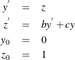
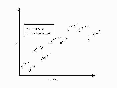
In a static solution, n–1 initial value problems are solved using the first n–1 data values as initial values. The equations
are integrated using the ![]() th data value as an initial value to the i+1 data value. Figure 19.48 displays a static simulation of noisy data from a simple differential equation. The static solution does not propagate errors
in initial values as the dynamic solution does.
th data value as an initial value to the i+1 data value. Figure 19.48 displays a static simulation of noisy data from a simple differential equation. The static solution does not propagate errors
in initial values as the dynamic solution does.
For estimation, the DYNAMIC and STATIC options in the FIT statement perform the same functions as they do in the SOLVE statement. Components of differential systems that have missing values or are not in the data set are simulated dynamically. For example, often in multiple compartment kinetic models, only one compartment is monitored. The differential equations that describe the unmonitored compartments are simulated dynamically.
For estimation, it is important to have accurate initial values for ODEs that are not in the data set. If an accurate initial value is not known, the initial value can be made an unknown parameter and estimated. This allows for errors in the initial values but increases the number of parameters to estimate by the number of equations.
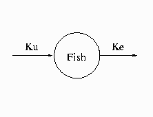
Consider the kinetic model for the accumulation of mercury (Hg) in mosquito fish (Matis, Miller, and Allen, 1991, p. 177). The model for this process is the one-compartment constant infusion model shown in Figure 19.49.
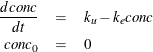
The differential equation that models this process is
The analytical solution to the model is
The data for the model are
data fish;
   input day conc;
datalines;
0.0    0.0
1.0    0.15
2.0    0.2
3.0    0.26
4.0    0.32
6.0    0.33
;
To fit this model in differential form, use the following statements:
proc model data=fish;
   parm ku ke;

   dert.conc = ku - ke * conc;

   fit conc / time=day;
run;
The results from this estimation are shown in Figure 19.50.
To perform a dynamic estimation of the differential equation, add the DYNAMIC option to the FIT statement.
proc model data=fish;
   parm ku .3 ke .3;

   dert.conc = ku - ke * conc;

   fit conc / time = day dynamic;
run;
The equation DERT.CONC is integrated from ![]() . The results from this estimation are shown in Figure 19.51.
. The results from this estimation are shown in Figure 19.51.
To perform a dynamic estimation of the differential equation and estimate the initial value, use the following statements:
proc model data=fish;
   parm ku .3 ke .3 conc0 0;

   dert.conc = ku - ke * conc;

   fit conc initial=(conc = conc0) / time = day dynamic;
run;
The INITIAL= option in the FIT statement is used to associate the initial value of a differential equation with a parameter. The results from this estimation are shown in Figure 19.52.
Finally, to estimate the fish model by using the analytical solution, use the following statements:
proc model data=fish;
   parm ku .3  ke .3;

   conc = (ku/ ke)*( 1 -exp(-ke * day));

   fit conc;
run;
The results from this estimation are shown in Figure 19.53.
A comparison of the results among the four estimations reveals that the two dynamic estimations and the analytical estimation give nearly identical results (identical to the default precision). The two dynamic estimations are identical because the estimated initial value (0.00013071) is very close to the initial value used in the first dynamic estimation (0). Note also that the static model did not require an initial guess for the parameter values. Static estimation, in general, is more forgiving of bad initial values.
The form of the estimation that is preferred depends mostly on the model and data. If a very accurate initial value is known, then a dynamic estimation makes sense. If, additionally, the model can be written analytically, then the analytical estimation is computationally simpler. If only an approximate initial value is known and not modeled as an unknown parameter, the static estimation is less sensitive to errors in the initial value.
The form of the error in the model is also an important factor in choosing the form of the estimation. If the error term is additive and independent of previous error, then the dynamic mode is appropriate. If, on the other hand, the errors are cumulative, a static estimation is more appropriate. See the section Monte Carlo Simulation for an example.
Auxiliary equations can be used with differential equations. These are equations that need to be satisfied with the differential equations at each point between each data value. They are automatically added to the system, so you do not need to specify them in the SOLVE or FIT statement.
Consider the following example.
The Michaelis-Menten equations describe the kinetics of an enzyme-catalyzed reaction. The enzyme is E, and S is called the substrate. The enzyme first reacts with the substrate to form the enzyme-substrate complex ES, which then breaks down in a second step to form enzyme and products P.
The reaction rates are described by the following system of differential equations:
![\begin{align*} \frac{d[\mi{ES}]}{dt} & = k_{1}([\mi{E}] - [\mi{ES}])[\mi{S}] - k_{2}[\mi{ES}] - k_{3}[\mi{ES}] \\ \frac{d[\mi{S}]}{dt} & = -k_{1}([\mi{E}] - [\mi{ES}])[\mi{S}] + k_{2}[\mi{ES}] \\ \lbrack \mi{E}\rbrack & = [\mi{E}]_{\mi{tot}} - [\mi{ES}] \end{align*}](images/etsug_model0423.png)
The first equation describes the rate of formation of ES from E + S. The rate of formation of ES from E + P is very small
and can be ignored. The enzyme is in either the complexed or the uncomplexed form. So if the total (![]() ) concentration of enzyme and the amount bound to the substrate is known,
) concentration of enzyme and the amount bound to the substrate is known, ![]() can be obtained by conservation.
can be obtained by conservation.
In this example, the conservation equation is an auxiliary equation and is coupled with the differential equations for integration.
You must provide a time variable in the data set. The name of the time variable defaults to TIME. You can use other variables as the time variable by specifying the TIME= option in the FIT or SOLVE statement. The time intervals need not be evenly spaced. If the time variable for the current observation is less than the time variable for the previous observation, the integration is restarted.
Consider the following differential equation
and the data set
data t2;
   y=0; time=0; output;
   y=2; time=1; output;
   y=3; time=2; output;
run;
The problem is to find values for X that satisfy the differential equation and the data in the data set. Problems of this kind are sometimes referred to as goal-seeking problems because they require you to search for values of X that satisfy the goal of Y.
This problem is solved with the following statements:
proc model data=t2;
   independent x 0;
   dependent y;
   parm a 5;
   dert.y = a * x;
   solve x / out=goaldata;
run;

proc print data=goaldata;
run;
The output from the PROC PRINT statement is shown in Figure 19.54.
Note that an initial value of 0 is provided for the X variable because it is undetermined at TIME = 0.
In the preceding goal-seeking example, X is treated as a linear function between each set of data points (see Figure 19.55).
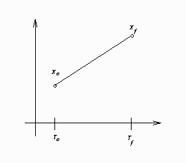
If you integrate ![]() manually, you have
manually, you have
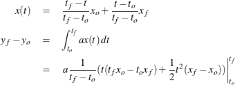
For observation 2, this reduces to
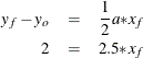
So ![]() for this observation.
for this observation.
Goal seeking for the TIME variable is not allowed.