The MODEL Procedure
- Dependent Regressors and Two-Stage Least Squares
- Seemingly Unrelated Regression
- Three-Stage Least Squares Estimation
- Generalized Method of Moments (GMM)
- Iterated Generalized Method of Moments (ITGMM)
- Simulated Method of Moments (SMM)
- Full Information Maximum Likelihood Estimation (FIML)
- Multivariate t Distribution Estimation
- t Distribution Details
- Empirical Distribution Estimation and Simulation
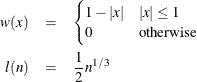
Consider the general nonlinear model:
where q ![]() is a real vector valued function of y
is a real vector valued function of y![]()
![]() , x
, x![]()
![]() ,
, ![]() , where g is the number of equations, l is the number of exogenous variables (lagged endogenous variables are considered exogenous here), p is the number of parameters, and t ranges from 1 to n.
, where g is the number of equations, l is the number of exogenous variables (lagged endogenous variables are considered exogenous here), p is the number of parameters, and t ranges from 1 to n. ![]()
![]() is a vector of instruments.
is a vector of instruments. ![]() is an unobservable disturbance vector with the following properties:
is an unobservable disturbance vector with the following properties:
All of the methods implemented in PROC MODEL aim to minimize an objective function. The following table summarizes the objective functions that define the estimators and the corresponding estimator of the covariance of the parameter estimates for each method.
Table 19.1: Summary of PROC MODEL Estimation Methods
|
Method |
Instruments |
Objective Function |
Covariance of |
|---|---|---|---|
|
OLS |
no |
|
|
|
ITOLS |
no |
|
|
|
SUR |
no |
|
|
|
ITSUR |
no |
|
|
|
N2SLS |
yes |
|
|
|
IT2SLS |
yes |
|
|
|
N3SLS |
yes |
|
|
|
IT3SLS |
yes |
|
|
|
GMM |
yes |
|
|
|
ITGMM |
yes |
|
|
|
FIML |
no |
|
|
|
|
The column labeled "Instruments" identifies the estimation methods that require instruments. The variables used in this table and the remainder of this chapter are defined as follows:
![]() is the number of nonmissing observations.
is the number of nonmissing observations.
![]() is the number of equations.
is the number of equations.
![]() is the number of instrumental variables.
is the number of instrumental variables.
![${\mb{r} = \left[\begin{matrix} r_{1} \\ r_{2} \\ {\vdots } \\ r_{g} \end{matrix}\right]}$](images/etsug_model0109.png) is the
is the ![]() vector of residuals for the g equations stacked together.
vector of residuals for the g equations stacked together.
![${\mb{r}_{i} = \left[\begin{matrix} q_{i}(\mb{y}_{1}, \mb{x}_{1}, \btheta ) \\ q_{i}(\mb{y}_{2}, \mb{x}_{2}, \btheta ) \\ \vdots \\ q_{i}(\mb{y}_{n}, \mb{x}_{n}, \btheta ) \end{matrix}\right]}$](images/etsug_model0111.png) is the
is the ![]() column vector of residuals for the i th equation.
column vector of residuals for the i th equation.
- S
-
is a
 matrix that estimates
  , the covariances of the errors across equations (referred to as the S matrix).
- X
-
is an
 matrix of partial derivatives of the residual with respect to the parameters.
- W
-
is an
 matrix,
  .
.
- Z
-
is an
 matrix of instruments.
- Y
-
is a
 matrix of instruments.
  .
.

-
 is an
is an  matrix.
  is a
is a  column vector obtained from stacking the columns of
- U
-
is an
 matrix of residual errors.
  .
.
- Q
-
is the
matrix  .
.
- Q

-
is an
matrix  .
.
- I
-
is an
identity matrix.
- J


-
is first moment of the crossproduct
 ,
,
- z
-
is a
 column vector of instruments for observation
  .
.  is also the th row of Z.

-
is the
 matrix that represents the variance of the moment functions.
- k
-
is the number of instrumental variables used.
- constant
-
is the constant
 .
.

-
is the notation for a Kronecker product.
All vectors are column vectors unless otherwise noted. Other estimates of the covariance matrix for FIML are also available.
Ordinary regression analysis is based on several assumptions. A key assumption is that the independent variables are in fact statistically independent of the unobserved error component of the model. If this assumption is not true (if the regressor varies systematically with the error), then ordinary regression produces inconsistent results. The parameter estimates are biased.
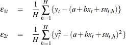
Regressors might fail to be independent variables because they are dependent variables in a larger simultaneous system. For this reason, the problem of dependent regressors is often called simultaneous equation bias. For example, consider the following two-equation system:
In the first equation, y![]() is a dependent, or endogenous, variable. As shown by the second equation, y
is a dependent, or endogenous, variable. As shown by the second equation, y![]() is a function of y
is a function of y![]() , which by the first equation is a function of
, which by the first equation is a function of ![]()
![]() , and therefore y
, and therefore y![]() depends on
depends on ![]()
![]() . Likewise, y
. Likewise, y![]() depends on
depends on ![]()
![]() and is a dependent regressor in the second equation. This is an example of a simultaneous equation system; y
and is a dependent regressor in the second equation. This is an example of a simultaneous equation system; y![]() and y
and y![]() are a function of all the variables in the system.
are a function of all the variables in the system.
Using the ordinary least squares (OLS) estimation method to estimate these equations produces biased estimates. One solution
to this problem is to replace y![]() and y
and y![]() on the right-hand side of the equations with predicted values, thus changing the regression problem to the following:
on the right-hand side of the equations with predicted values, thus changing the regression problem to the following:
This method requires estimating the predicted values ![]() and
and ![]() through a preliminary, or "first stage," instrumental regression. An instrumental regression is a regression of the dependent regressors on a set of instrumental variables, which can be any independent variables useful for predicting the dependent regressors. In this example, the equations are
linear and the exogenous variables for the whole system are known. Thus, the best choice for instruments (of the variables
in the model) are the variables x
through a preliminary, or "first stage," instrumental regression. An instrumental regression is a regression of the dependent regressors on a set of instrumental variables, which can be any independent variables useful for predicting the dependent regressors. In this example, the equations are
linear and the exogenous variables for the whole system are known. Thus, the best choice for instruments (of the variables
in the model) are the variables x![]() and x
and x![]() .
.
This method is known as two-stage least squares or 2SLS, or more generally as the instrumental variables method. The 2SLS method for linear models is discussed in Pindyck and Rubinfeld (1981, pp. 191–192). For nonlinear models this situation is more complex, but the idea is the same. In nonlinear 2SLS, the derivatives of the model with respect to the parameters are replaced with predicted values. See the section Choice of Instruments for further discussion of the use of instrumental variables in nonlinear regression.
To perform nonlinear 2SLS estimation with PROC MODEL, specify the instrumental variables with an INSTRUMENTS statement and specify the 2SLS or N2SLS option in the FIT statement. The following statements show how to estimate the first equation in the preceding example with PROC MODEL:
   proc model data=in;
      y1 = a1 + b1 * y2 + c1 * x1;
      fit y1 / 2sls;
      instruments x1 x2;
   run;
The 2SLS or instrumental variables estimator can be computed by using a first-stage regression on the instrumental variables
as described previously. However, PROC MODEL actually uses the equivalent but computationally more appropriate technique of
projecting the regression problem into the linear space defined by the instruments. Thus, PROC MODEL does not produce any
"first stage" results when you use 2SLS. If you specify the FSRSQ option in the FIT statement, PROC MODEL prints "First-Stage R![]() " statistic for each parameter estimate.
" statistic for each parameter estimate.
Formally, the ![]() that minimizes
that minimizes
is the N2SLS estimator of the parameters. The estimate of ![]() at the final iteration is used in the covariance of the parameters given in Table 19.1. See Amemiya (1985, p. 250) for details on the properties of nonlinear two-stage least squares.
at the final iteration is used in the covariance of the parameters given in Table 19.1. See Amemiya (1985, p. 250) for details on the properties of nonlinear two-stage least squares.
If the regression equations are not simultaneous (so there are no dependent regressors), seemingly unrelated regression (SUR) can be used to estimate systems of equations with correlated random errors. The large-sample efficiency of an estimation
can be improved if these cross-equation correlations are taken into account. SUR is also known as joint generalized least squares or Zellner regression. Formally, the ![]() that minimizes
that minimizes
is the SUR estimator of the parameters.
The SUR method requires an estimate of the cross-equation covariance matrix, ![]() . PROC MODEL first performs an OLS estimation, computes an estimate,
. PROC MODEL first performs an OLS estimation, computes an estimate, ![]() , from the OLS residuals, and then performs the SUR estimation based on
, from the OLS residuals, and then performs the SUR estimation based on ![]() . The OLS results are not printed unless you specify the OLS option in addition to the SUR option.
. The OLS results are not printed unless you specify the OLS option in addition to the SUR option.
You can specify the ![]() to use for SUR by storing the matrix in a SAS data set and naming that data set in the SDATA= option. You can also feed the
to use for SUR by storing the matrix in a SAS data set and naming that data set in the SDATA= option. You can also feed the ![]() computed from the SUR residuals back into the SUR estimation process by specifying the ITSUR option. You can print the estimated
covariance matrix
computed from the SUR residuals back into the SUR estimation process by specifying the ITSUR option. You can print the estimated
covariance matrix ![]() by using the COVS option in the FIT statement.
by using the COVS option in the FIT statement.
The SUR method requires estimation of the ![]() matrix, and this increases the sampling variability of the estimator for small sample sizes. The efficiency gain that SUR
has over OLS is a large sample property, and you must have a reasonable amount of data to realize this gain. For a more detailed
discussion of SUR, see Pindyck and Rubinfeld (1981, pp. 331–333).
matrix, and this increases the sampling variability of the estimator for small sample sizes. The efficiency gain that SUR
has over OLS is a large sample property, and you must have a reasonable amount of data to realize this gain. For a more detailed
discussion of SUR, see Pindyck and Rubinfeld (1981, pp. 331–333).
If the equation system is simultaneous, you can combine the 2SLS and SUR methods to take into account both dependent regressors and cross-equation correlation of the errors. This is called three-stage least squares (3SLS).
Formally, the ![]() that minimizes
that minimizes
is the 3SLS estimator of the parameters. For more details on 3SLS, see Gallant (1987, p. 435).
Residuals from the 2SLS method are used to estimate the ![]() matrix required for 3SLS. The results of the preliminary 2SLS step are not printed unless the 2SLS option is also specified.
matrix required for 3SLS. The results of the preliminary 2SLS step are not printed unless the 2SLS option is also specified.
To use the three-stage least squares method, specify an INSTRUMENTS statement and use the 3SLS or N3SLS option in either the PROC MODEL statement or a FIT statement.
For systems of equations with heteroscedastic errors, generalized method of moments (GMM) can be used to obtain efficient estimates of the parameters. See the section Heteroscedasticity for alternatives to GMM.
Consider the nonlinear model
where ![]() is a vector of instruments and
is a vector of instruments and ![]() is an unobservable disturbance vector that can be serially correlated and nonstationary.
is an unobservable disturbance vector that can be serially correlated and nonstationary.
In general, the following orthogonality condition is desired:
This condition states that the expected crossproducts of the unobservable disturbances, ![]() , and functions of the observable variables are set to 0. The first moment of the crossproducts is
, and functions of the observable variables are set to 0. The first moment of the crossproducts is
where ![]() .
.
The case where ![]() is considered here, where p is the number of parameters.
is considered here, where p is the number of parameters.
Estimate the true parameter vector ![]() by the value of
by the value of ![]() that minimizes
that minimizes
The parameter vector that minimizes this objective function is the GMM estimator. GMM estimation is requested in the FIT statement with the GMM option.
The variance of the moment functions, ![]() , can be expressed as
, can be expressed as
![\begin{eqnarray*} {\bV } & =& E \left(\sum _{t=1}^{n}{\bepsilon _{t} {\otimes } \Strong{z}_{t}}\right) \left(\sum _{s=1}^{n}{\bepsilon _{s} {\otimes } \Strong{z}_{s}}\right)’ \\ & =& \sum _{t=1}^{n} \sum _{s=1}^{n}{E \left[ (\bepsilon _{t} {\otimes } \Strong{z}_{t}) ( \bepsilon _{s} {\otimes } \Strong{z}_{s})’\right]} \\ & =& n {\bS }_{n}^{0} \nonumber \end{eqnarray*}](images/etsug_model0167.png)
where ![]() is estimated as
is estimated as
Note that ![]() is a
is a ![]() matrix. Because Var
matrix. Because Var ![]() does not decrease with increasing n, you consider estimators of
does not decrease with increasing n, you consider estimators of ![]() of the form:
of the form:
![\begin{eqnarray*} \hat{{\bS }}_{n}(l(n)) & =& \sum _{{\tau } = -n + 1}^{n-1}{\hat{w} ( \frac{\tau }{l(n)} ) {\bD } \hat{{\bS }}_{n,{\tau }}} {\bD } \\ \hat{{\bS }}_{n,{\tau }} & =& \begin{cases} \sum \limits _{t=1+{\tau }}^{n}{[\Strong{q} (\Strong{y}_{t}, \Strong{x}_{t},{\btheta }^{\# }) {\otimes }\Strong{z}_{t}][\Strong{q} (\Strong{y}_{t-{\tau }}, \Strong{x}_{t-{\tau }}, {\btheta }^{\# }){\otimes }\Strong{z}_{t-{\tau }}]’} & {\tau }\ge 0 \\ (\hat{{\bS }}_{n,-{\tau }})’ & {\tau }<0 \end{cases}\\ \hat{w}(\frac{\tau }{l(n)}) & =& \begin{cases} w(\frac{\tau }{l(n)}) & l(n) > 0 \\ \delta _{\tau ,0} & l(n) = 0 \end{cases} \nonumber \end{eqnarray*}](images/etsug_model0173.png)
where ![]() is a scalar function that computes the bandwidth parameter,
is a scalar function that computes the bandwidth parameter, ![]() is a scalar valued kernel, and the Kronecker delta function,
is a scalar valued kernel, and the Kronecker delta function, ![]() , is 1 if
, is 1 if ![]() and 0 otherwise. The diagonal matrix
and 0 otherwise. The diagonal matrix ![]() is used for a small sample degrees of freedom correction (Gallant, 1987). The initial
is used for a small sample degrees of freedom correction (Gallant, 1987). The initial ![]() used for the estimation of
used for the estimation of ![]() is obtained from a 2SLS estimation of the system. The degrees of freedom correction is handled by the VARDEF= option as it is for the S matrix estimation.
is obtained from a 2SLS estimation of the system. The degrees of freedom correction is handled by the VARDEF= option as it is for the S matrix estimation.
The following kernels are supported by PROC MODEL. They are listed with their default bandwidth functions.
Bartlett: KERNEL=BART
Parzen: KERNEL=PARZEN
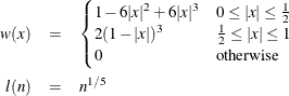
Quadratic spectral: KERNEL=QS
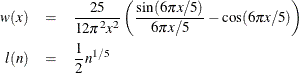

Details of the properties of these and other kernels are given in Andrews (1991). Kernels are selected with the KERNEL= option; KERNEL=PARZEN is the default. The general form of the KERNEL= option is
KERNEL=( PARZEN | QS | BART, c, e )
where the ![]() and
and ![]() are used to compute the bandwidth parameter as
are used to compute the bandwidth parameter as
The bias of the standard error estimates increases for large bandwidth parameters. A warning message is produced for bandwidth
parameters greater than ![]() . For a discussion of the computation of the optimal
. For a discussion of the computation of the optimal ![]() , refer to Andrews (1991).
, refer to Andrews (1991).
The "Newey-West" kernel (Newey and West, 1987) corresponds to the Bartlett kernel with bandwidth parameter ![]() . That is, if the "lag length" for the Newey-West kernel is
. That is, if the "lag length" for the Newey-West kernel is ![]() , then the corresponding MODEL procedure syntax is KERNEL=(bart, L+1, 0).
, then the corresponding MODEL procedure syntax is KERNEL=(bart, L+1, 0).
Andrews and Monahan (1992) show that using prewhitening in combination with GMM can improve confidence interval coverage and reduce over rejection of t statistics at the cost of inflating the variance and MSE of the estimator. Prewhitening can be performed by using the %AR macros.
For the special case that the errors are not serially correlated—that is,
the estimate for ![]() reduces to
reduces to
The option KERNEL=(kernel,0,) is used to select this type of estimation when using GMM.
The covariance of GMM estimators, given a general weighting matrix ![]() , is
, is
By default or when GENGMMV is specified, this is the covariance of GMM estimators.
If the weighting matrix is the same as ![]() , then the covariance of GMM estimators becomes
, then the covariance of GMM estimators becomes
If NOGENGMMV is specified, this is used as the covariance estimators.
Let r be the number of unique instruments times the number of equations. The value r represents the number of orthogonality conditions imposed by the GMM method. Under the assumptions of the GMM method, ![]() linearly independent combinations of the orthogonality should be close to zero. The GMM estimates are computed by setting
these combinations to zero. When r exceeds the number of parameters to be estimated, the OBJECTIVE*N, reported at the end of the estimation, is an asymptotically
valid statistic to test the null hypothesis that the overidentifying restrictions of the model are valid. The OBJECTIVE*N
is distributed as a chi-square with
linearly independent combinations of the orthogonality should be close to zero. The GMM estimates are computed by setting
these combinations to zero. When r exceeds the number of parameters to be estimated, the OBJECTIVE*N, reported at the end of the estimation, is an asymptotically
valid statistic to test the null hypothesis that the overidentifying restrictions of the model are valid. The OBJECTIVE*N
is distributed as a chi-square with ![]() degrees of freedom (Hansen, 1982, p. 1049). When the GMM method is selected, the value of the overidentifying restrictions test statistic, also known as Hansen’s
J test statistic, and its associated number of degrees of freedom are reported together with the probability under the null
hypothesis.
degrees of freedom (Hansen, 1982, p. 1049). When the GMM method is selected, the value of the overidentifying restrictions test statistic, also known as Hansen’s
J test statistic, and its associated number of degrees of freedom are reported together with the probability under the null
hypothesis.
Iterated generalized method of moments is similar to the iterated versions of 2SLS, SUR, and 3SLS. The variance matrix for GMM estimation is reestimated at each iteration with the parameters determined by the GMM estimation. The iteration terminates when the variance matrix for the equation errors change less than the CONVERGE= value. Iterated generalized method of moments is selected by the ITGMM option on the FIT statement. For some indication of the small sample properties of ITGMM, see Ferson and Foerster (1993).
The SMM method uses simulation techniques in model inference and estimation. It is appropriate for estimating models in which integrals appear in the objective function, and these integrals can be approximated by simulation. There might be various reasons for integrals to appear in an objective function (for example, transformation of a latent model into an observable model, missing data, random coefficients, heterogeneity, and so on).
This simulation method can be used with all the estimation methods except full information maximum likelihood (FIML) in PROC MODEL. SMM, also known as simulated generalized method of moments (SGMM), is the default estimation method because of its nice properties.
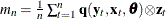
A general nonlinear model can be described as
where q ![]() is a real vector valued function of y
is a real vector valued function of y ![]()
![]() , x
, x ![]()
![]() ,
, ![]() ; g is the number of equations; l is the number of exogenous variables (lagged endogenous variables are considered exogenous here); p is the number of parameters; and t ranges from 1 to n.
; g is the number of equations; l is the number of exogenous variables (lagged endogenous variables are considered exogenous here); p is the number of parameters; and t ranges from 1 to n. ![]() is an unobservable disturbance vector with the following properties:
is an unobservable disturbance vector with the following properties:
In many cases, it is not possible to write ![]() in a closed form. Instead
in a closed form. Instead ![]() is expressed as an integral of a function
is expressed as an integral of a function ![]() ; that is,
; that is,
where f ![]() is a real vector valued function of y
is a real vector valued function of y ![]()
![]() , x
, x ![]()
![]() ,
, ![]() , and u
, and u ![]()
![]() , m is the number of stochastic variables with a known distribution
, m is the number of stochastic variables with a known distribution ![]() . Since the distribution of u is completely known, it is possible to simulate artificial draws from this distribution. Using such independent draws
. Since the distribution of u is completely known, it is possible to simulate artificial draws from this distribution. Using such independent draws ![]() ,
, ![]() , and the strong law of large numbers,
, and the strong law of large numbers, ![]() can be approximated by
can be approximated by
Generalized method of moments (GMM) is widely used to obtain efficient estimates for general model systems. When the moment
conditions are not readily available in closed forms but can be approximated by simulation, simulated generalized method of
moments (SGMM) can be used. The SGMM estimators have the nice property of being asymptotically consistent and normally distributed
even if the number of draws ![]() is fixed (see McFadden 1989; Pakes and Pollard 1989).
is fixed (see McFadden 1989; Pakes and Pollard 1989).
Consider the nonlinear model
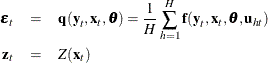
where ![]() is a vector of k instruments and
is a vector of k instruments and ![]() is an unobservable disturbance vector that can be serially correlated and nonstationary. In the case of no instrumental variables,
is an unobservable disturbance vector that can be serially correlated and nonstationary. In the case of no instrumental variables,
![]() is 1.
is 1. ![]() is the vector of moment conditions, and it is approximated by simulation.
is the vector of moment conditions, and it is approximated by simulation.
In general, theory suggests the following orthogonality condition
which states that the expected crossproducts of the unobservable disturbances, ![]() , and functions of the observable variables are set to 0. The sample means of the crossproducts are
, and functions of the observable variables are set to 0. The sample means of the crossproducts are
where ![]() . The case where
. The case where ![]() , where p is the number of parameters, is considered here. An estimate of the true parameter vector
, where p is the number of parameters, is considered here. An estimate of the true parameter vector ![]() is the value of
is the value of ![]() that minimizes
that minimizes
The steps for SGMM are as follows:
1. Start with a positive definite ![]() matrix. This
matrix. This ![]() matrix can be estimated from a consistent estimator of
matrix can be estimated from a consistent estimator of ![]() . If
. If ![]() is a consistent estimator, then
is a consistent estimator, then ![]() for
for ![]() can be simulated
can be simulated ![]() number of times. A consistent estimator of
number of times. A consistent estimator of ![]() is obtained as
is obtained as
![]() must be large so that this is an consistent estimator of
must be large so that this is an consistent estimator of ![]() .
.
2. Simulate ![]() number of
number of ![]() for
for ![]() . As shown by Gourieroux and Monfort (1993), the number of simulations
. As shown by Gourieroux and Monfort (1993), the number of simulations ![]() does not need to be very large. For
does not need to be very large. For ![]() , the SGMM estimator achieves 90% of the efficiency of the corresponding GMM estimator. Find
, the SGMM estimator achieves 90% of the efficiency of the corresponding GMM estimator. Find ![]() that minimizes the quadratic product of the moment conditions again with the weight matrix being
that minimizes the quadratic product of the moment conditions again with the weight matrix being ![]() .
.
3. The covariance matrix of ![]() is given as (Gourieroux and Monfort, 1993)
is given as (Gourieroux and Monfort, 1993)
where ![]() ,
, ![]() is the matrix of partial derivatives of the residuals with respect to the parameters,
is the matrix of partial derivatives of the residuals with respect to the parameters, ![]() is the covariance of moments from estimated parameters
is the covariance of moments from estimated parameters ![]() , and
, and ![]() is the covariance of moments for each observation from simulation. The first term is the variance-covariance matrix of the
exact GMM estimator, and the second term accounts for the variation contributed by simulating the moments.
is the covariance of moments for each observation from simulation. The first term is the variance-covariance matrix of the
exact GMM estimator, and the second term accounts for the variation contributed by simulating the moments.
In PROC MODEL, if the user specifies the GMM and NDRAW options in the FIT statement, PROC MODEL first fits the model by using
N2SLS and computes ![]() by using the estimates from N2SLS and
by using the estimates from N2SLS and ![]() simulation. If NO2SLS is specified in the FIT statement,
simulation. If NO2SLS is specified in the FIT statement, ![]() is read from VDATA= data set. If the user does not provide a
is read from VDATA= data set. If the user does not provide a ![]() matrix, the initial starting value of
matrix, the initial starting value of ![]() is used as the estimator for computing the
is used as the estimator for computing the ![]() matrix in step 1. If ITGMM option is specified instead of GMM, then PROC MODEL iterates from step 1 to step 3 until the
matrix in step 1. If ITGMM option is specified instead of GMM, then PROC MODEL iterates from step 1 to step 3 until the ![]() matrix converges.
matrix converges.
The consistency of the parameter estimates is not affected by the variance correction shown in the second term in step 3.
The correction on the variance of parameter estimates is not computed by default. To add the adjustment, use ADJSMMV option
on the FIT statement. This correction is of the order of ![]() and is small even for moderate
and is small even for moderate ![]() .
.
The following example illustrates how to use SMM to estimate a simple regression model. Suppose the model is
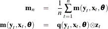
First, consider the problem in a GMM context. The first two moments of y are easily derived:
Rewrite the moment conditions in the form similar to the discussion above:
Then you can estimate this model by using GMM with following statements:
   proc model data=a;
      parms a b s;
      instrument x;
      eq.m1 = y-(a+b*x);
      eq.m2 = y*y - (a+b*x)**2 - s*s;
      bound s > 0;
      fit m1 m2 / gmm;
   run;
Now suppose you do not have the closed form for the moment conditions. Instead you can simulate the moment conditions by generating
![]() number of simulated samples based on the parameters. Then the simulated moment conditions are
number of simulated samples based on the parameters. Then the simulated moment conditions are
This model can be estimated by using SGMM with the following statements:
   proc model data=_tmpdata;
      parms a b s;
      instrument x;
      ysim = (a+b*x) + s * rannor( 98711 );
      eq.m1 = y-ysim;
      eq.m2 = y*y - ysim*ysim;
      bound s > 0;
      fit m1 m2 / gmm ndraw=10;
   run;
You can use the following MOMENT statement instead of specifying the two moment equations above:
moment ysim=(1, 2);
In cases where you require a large number of moment equations, using the MOMENT statement to specify them is more efficient.
Note that the NDRAW= option tells PROC MODEL that this is a simulation-based estimation. Thus, the random number function
RANNOR returns random numbers in estimation process. During the simulation, 10 draws of ![]() and
and ![]() are generated for each observation, and the averages enter the objective functions just as the equations specified previously.
are generated for each observation, and the averages enter the objective functions just as the equations specified previously.
The simulation method can be used not only with GMM and ITGMM, but also with OLS, ITOLS, SUR, ITSUR, N2SLS, IT2SLS, N3SLS,
and IT3SLS. These simulation-based methods are similar to the corresponding methods in PROC MODEL; the only difference is
that the objective functions include the average of the ![]() simulations.
simulations.
A different approach to the simultaneous equation bias problem is the full information maximum likelihood (FIML) estimation method (Amemiya, 1977).
Compared to the instrumental variables methods (2SLS and 3SLS), the FIML method has these advantages and disadvantages:
-
FIML does not require instrumental variables.
-
FIML requires that the model include the full equation system, with as many equations as there are endogenous variables. With 2SLS or 3SLS, you can estimate some of the equations without specifying the complete system.
-
FIML assumes that the equations errors have a multivariate normal distribution. If the errors are not normally distributed, the FIML method might produce poor results. 2SLS and 3SLS do not assume a specific distribution for the errors.
-
The FIML method is computationally expensive.
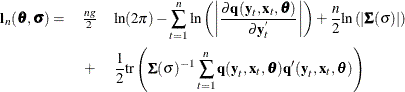
The full information maximum likelihood estimators of ![]() and
and ![]() are the
are the ![]() and
and ![]() that minimize the negative log-likelihood function:
that minimize the negative log-likelihood function:
The option FIML requests full information maximum likelihood estimation. If the errors are distributed normally, FIML produces
efficient estimators of the parameters. If instrumental variables are not provided, the starting values for the estimation
are obtained from a SUR estimation. If instrumental variables are provided, then the starting values are obtained from a 3SLS
estimation. The log-likelihood value and the l![]() norm of the gradient of the negative log-likelihood function are shown in the estimation summary.
norm of the gradient of the negative log-likelihood function are shown in the estimation summary.
To compute the minimum of ![]() , this function is concentrated using the relation
, this function is concentrated using the relation
This results in the concentrated negative log-likelihood function discussed in Davidson and MacKinnon (1993):
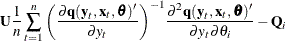
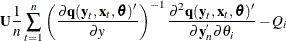
The gradient of the negative log-likelihood function is
![\begin{eqnarray*} {\nabla }_{i}(t) & =& -\textrm{tr} \left( \left( \frac{{\partial }\Strong{q} (\Strong{y}_{t}, \Strong{x}_{t}, \btheta )}{{\partial } \Strong{y}_{t}^{'}} \right)^{-1} \frac{{\partial }^{2}\Strong{q} (\Strong{y}_{t}, \Strong{x}_{t},\btheta )}{{\partial } \Strong{y}_{t}^{'} {\partial } \theta _{i}} \right) \\ & +& \frac{1}{2} \textrm{tr} \left( \bSigma (\theta )^{-1} ~ \frac{{\partial }{\bSigma }(\theta )}{{\partial } \theta _{i}} \right. \\ & & \left. \left[ I - {\bSigma }(\theta )^{-1} \Strong{q} (\Strong{y}_{t}, \Strong{x}_{t}, \btheta ) \Strong{q} (\Strong{y}_{t}, \Strong{x}_{t}, \btheta )’ \right] \right) \\ & +& \Strong{q} (\Strong{y}_{t}, \Strong{x}_{t}, \btheta ’) {\bSigma }(\theta )^{-1} \frac{{\partial }\Strong{q} (\Strong{y}_{t}, \Strong{x}_{t}, \btheta )}{{\partial } \theta _{i}} \end{eqnarray*}](images/etsug_model0238.png)
where
The estimator of the variance-covariance of ![]() (COVB) for FIML can be selected with the COVBEST= option with the following arguments:
(COVB) for FIML can be selected with the COVBEST= option with the following arguments:
- CROSS
-
selects the crossproducts estimator of the covariance matrix (Gallant, 1987, p. 473):
- GLS
-
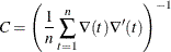
selects the generalized least squares estimator of the covariance matrix. This is computed as (Dagenais, 1978)
![\[ C = [ \hat{{\bZ }} ’ ( {\bSigma }(\theta )^{-1} {\otimes } I) \hat{{\bZ }}]^{-1} \]](images/etsug_model0242.png)
where
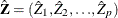 is and each column vector is obtained from stacking the columns of
 is an
is an  matrix of residuals and
  is an matrix .
- FDA
-
selects the inverse of concentrated likelihood Hessian as an estimator of the covariance matrix. The Hessian is computed numerically, so for a large problem this is computationally expensive.
The HESSIAN= option controls which approximation to the Hessian is used in the minimization procedure. Alternate approximations are used to improve convergence and execution time. The choices are as follows:
- CROSS
-
The crossproducts approximation is used.
- GLS
-
The generalized least squares approximation is used (default).
- FDA
-
The Hessian is computed numerically by finite differences.
HESSIAN=GLS has better convergence properties in general, but COVBEST=CROSS produces the most pessimistic standard error bounds.
When the HESSIAN= option is used, the default estimator of the variance-covariance of ![]() is the inverse of the Hessian selected.
is the inverse of the Hessian selected.
The multivariate t distribution is specified by using the ERRORMODEL statement with the T option. Other method specifications (FIML and OLS, for example ) are ignored when the ERRORMODEL statement is used for a distribution other than normal.
The probability density function for the multivariate t distribution is
![\[ P_ q = \frac{\Gamma ( \frac{df +m}{2} ) }{ (\pi * df)^{\frac{m}{2}} * \Gamma ( \frac{df}{2} ) \left| \bSigma (\sigma ) \right|^{\frac{1}{2}} } * \left( 1 + \frac{\mb{q} '(\mb{y}_{t}, \mb{x}_{t} , \btheta ) \bSigma (\sigma )^{-1} \mb{q} (\mb{y}_{t} , \mb{x}_{t}, \btheta )}{df} \right)^{-\frac{df+m}{2} } \]](images/etsug_model0248.png)
where m is the number of equations and ![]() is the degrees of freedom.
is the degrees of freedom.
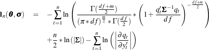
The maximum likelihood estimators of ![]() and
and ![]() are the
are the ![]() and
and ![]() that minimize the negative log-likelihood function:
that minimize the negative log-likelihood function:
The ERRORMODEL statement is used to request the t distribution maximum likelihood estimation. An OLS estimation is done to obtain initial parameter estimates and MSE.var estimates. Use NOOLS to turn off this initial estimation. If the errors are distributed normally, t distribution estimation produces results similar to FIML.
The multivariate model has a single shared degrees-of-freedom parameter, which is estimated. The degrees-of-freedom parameter
can also be set to a fixed value. The log-likelihood value and the l![]() norm of the gradient of the negative log-likelihood function are shown in the estimation summary.
norm of the gradient of the negative log-likelihood function are shown in the estimation summary.
Since a variance term is explicitly specified by using the ERRORMODEL statement, ![]() is estimated as a correlation matrix and
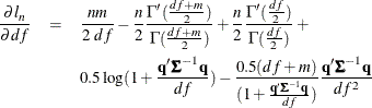
is estimated as a correlation matrix and ![]() is normalized by the variance. The gradient of the negative log-likelihood function with respect to the degrees of freedom
is
is normalized by the variance. The gradient of the negative log-likelihood function with respect to the degrees of freedom
is
The gradient of the negative log-likelihood function with respect to the parameters is
![\[ \frac{\partial l_ n}{\partial \theta _ i} = \frac{0.5 (df + m)}{(1 +\mb{q} '\bSigma ^{-1} \mb{q} /df)} \left[\frac{(2 ~ \mb{q} '\bSigma ^{-1} \frac{\partial \mb{q} }{\partial \theta _ i} )}{df} + \mb{q} ’ \bSigma ^{-1} \frac{\partial \bSigma }{\partial \theta _ i} \bSigma ^{-1} \mb{q} \right] - \frac{n}{2} \mr{trace} ( \bSigma ^{-1} \frac{\partial \bSigma }{\partial \theta _ i}) \]](images/etsug_model0253.png)
where
and
The estimator of the variance-covariance of ![]() (COVB) for the t distribution is the inverse of the likelihood Hessian. The gradient is computed analytically, and the Hessian is computed
numerically.
(COVB) for the t distribution is the inverse of the likelihood Hessian. The gradient is computed analytically, and the Hessian is computed
numerically.
The following SAS statements fit a model that uses least squares as the likelihood function, but represent the distribution of the residuals with an empirical cumulative distribution function (CDF). The plot of the empirical probability distribution is shown in Figure 19.24.
data t;  /* Sum of two normals  */
   format date monyy.;
   do t = 0 to 9.9 by 0.1;
      date = intnx( 'month', '1jun90'd, (t*10)-1 );
      y =  0.1 * (rannor(123)-10) +
            .5 * (rannor(123)+10);
      output;
   end;
run;
ods select Model.Liklhood.ResidSummary
           Model.Liklhood.ParameterEstimates;

proc model data=t time=t itprint;
   dependent y;
   parm a 5;

   y = a;
   obj = resid.y * resid.y;
   errormodel y ~ general( obj )
   cdf=(empirical=(tails=( normal percent=10)));

   fit y / outsn=s out=r;
   id  date;

   solve y / data=t(where=(date='1aug98'd))
             residdata=r sdata=s
             random=200 seed=6789 out=monte ;
run;


proc kde data=monte;
   univar y / plots=density;
run;
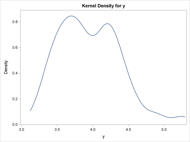
For simulation, if the CDF for the model is not built in to the procedure, you can use the CDF=EMPIRICAL() option. This uses the sorted residual data to create an empirical CDF. For computing the inverse CDF, the program needs to know how to handle the tails. For continuous data, the tail distribution is generally poorly determined. To counter this, the PERCENT= option specifies the percentage of the observations to use in constructing each tail. The default for the PERCENT= option is 10.
A normal distribution or a t distribution is used to extrapolate the tails to infinity. The standard errors for this extrapolation are obtained from the data so that the empirical CDF is continuous.