The MODEL Procedure

Solving Simultaneous Nonlinear Equation Systems

You can use a SOLVE statement to solve the nonlinear equation system for some variables when the values of other variables are given.

Consider the supply and demand model shown in the preceding example. The following statement computes equilibrium price (EEGP) and quantity (EEC) values for given observed cost (CCIUTC) values and stores them in the output data set EQUILIB.

title1 'Supply-Demand Model using General-form Equations';
proc model data=sashelp.citimon(where=(eec ne .));
   endogenous eegp eec;
   exogenous exvus cciutc;
   parameters a1 a2 a3 b1 b2 ;
   label eegp   = 'Gasoline Retail Price'
         eec    = 'Energy Consumption'
         cciutc = 'Consumer Debt';

   /* -------- Supply equation ------------- */
   eq.supply = eec - (a1 + a2 * eegp + a3 * cciutc);

   /* -------- Demand equation ------------- */
   eq.demand = eec - (b1 + b2 * eegp );

   /* -------- Instrumental variables -------*/
   lageegp = lag(eegp); lag2eegp=lag2(eegp);

   /* -------- Estimate parameters --------- */
   instruments _EXOG_ lageegp lag2eegp;
   fit supply demand / n3sls ;
   solve eegp eec / out=equilib;
run;

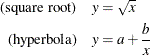
As a second example, suppose you want to compute points of intersection between the square root function and hyperbolas of the form ${a+b/x}$ . That is, you want to solve the system:

$\begin{align*} \text {(square root)}\quad y & = \sqrt {x} \\ \text {(hyperbola)} \quad y & = a + \frac{b}{x} \end{align*}$

The following statements read parameters for several hyperbolas in the input data set TEST and solve the nonlinear equations. The SOLVEPRINT option in the SOLVE statement prints the solution values. The ID statement is used to include the values of A and B in the output of the SOLVEPRINT option.

title1 'Solving a Simultaneous System';
data test;
   input a b @@;
datalines;
  0 1   1 1   1 2
;

proc model data=test;
   eq.sqrt      = sqrt(x) - y;
   eq.hyperbola = a + b / x - y;
   solve x y / solveprint;
   id a b;
run;

The printed output produced by this example consists of a model summary report, a listing of the solution values for each observation, and a solution summary report. The model summary for this example is shown in Figure 19.9.

Figure 19.9: Model Summary Report

Solving a Simultaneous System

The MODEL Procedure

Model Summary
Model Variables	2
ID Variables	2
Equations	2
Number of Statements	2

Model Variables	x y
Equations	sqrt hyperbola

The output produced by the SOLVEPRINT option is shown in Figure 19.10.

Figure 19.10: Solution Values for Each Observation

Solving a Simultaneous System

The MODEL Procedure

Simultaneous Simulation

Observation	1	a	0	b	1.0000	eq.hyperbola	0.000000
		Iterations	17	CC	0.000000

Solution Values
x	y
1.000000	1.000000

Observation	2	a	1.0000	b	1.0000	eq.hyperbola	0.000000
		Iterations	5	CC	0.000000

Solution Values
x	y
2.147899	1.465571

Observation	3	a	1.0000	b	2.0000	eq.hyperbola	0.000000
		Iterations	4	CC	0.000000

Solution Values
x	y
2.875130	1.695621

For each observation, a heading line is printed that lists the values of the ID variables for the observation and information about the iterative process used to compute the solution. The number of iterations required, and the convergence measure (labeled CC) are printed. This convergence measure indicates the maximum error by which solution values fail to satisfy the equations. When this error is small enough (as determined by the CONVERGE= option), the iterations terminate. The equation with the largest error is indicated. For example, for observation 3 the HYPERBOLA equation has an error of ${4.42{\times }10^{-13}}$ while the error of the SQRT equation is even smaller. Following the heading line for the observation, the solution values are printed.

The last part of the SOLVE statement output is the solution summary report shown in Figure 19.11. This report summarizes the solution method used (Newton’s method by default), the iteration history, and the observations processed.

Figure 19.11: Solution Summary Report

Solving a Simultaneous System

The MODEL Procedure

Simultaneous Simulation

Data Set Options
DATA=	TEST

Solution Summary
Variables Solved	2
Implicit Equations	2
Solution Method	NEWTON
CONVERGE=	1E-8
Maximum CC	9.176E-9
Maximum Iterations	17
Total Iterations	26
Average Iterations	8.666667

Observations Processed
Read	3
Solved	3

Variables Solved For	x y
Equations Solved	sqrt hyperbola