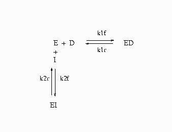
Example 19.10 Systems of Differential Equations :: SAS/ETS(R) 12.3 User's Guide

Example 19.10 Systems of Differential Equations

The following is a simplified reaction scheme for the competitive inhibitors with recombinant human renin (Morelock et al. 1995).

Output 19.10.1: Competitive Inhibition of Recombinant Human Renin

modsim

In Output 19.10.1, E=enzyme, D=probe, and I=inhibitor.

The differential equations that describe this reaction scheme are as follows:

$\frac{d\mi {D} }{dt} = k1r{\ast }\mi {ED} - k1f {\ast }\mi {E} {\ast }\mi {D}$

$\frac{d\mi {ED} }{dt} = k1f{\ast } \mi {E} {\ast }\mi {D} - k1r{\ast }\mi {ED}$

$\frac{d\mi {E} }{dt} = k1r{\ast } \mi {ED} - k1f{\ast } \mi {E} {\ast } \mi {D} + k2r {\ast } \mi {EI} - k2f {\ast } \mi {E} {\ast }\mi {I}$

$\frac{d\mi {EI} }{dt} = k2f{\ast } \mi {E} {\ast }\mi {I} - k2r {\ast } \mi {EI}$

$\frac{d\mi {I} }{dt} = k2r{\ast } \mi {EI} - k2f {\ast } \mi {E} {\ast } \mi {I}$

For this system, the initial values for the concentrations are derived from equilibrium considerations (as a function of parameters) or are provided as known values.

The experiment used to collect the data was carried out in two ways; preincubation (type='disassoc') and no preincubation (type='assoc'). The data also contain repeated measurements. The data contain values for fluorescence F, which is a function of concentration. Since there are no direct data for the concentrations, all the differential equations are simulated dynamically.

The SAS statements used to fit this model are as follows:

title1 'Systems of Differential Equations Example';

proc sort data=fit;
   by type time;
run;

%let k1f = 6.85e6  ;
%let k1r = 3.43e-4 ;
%let k2f = 1.8e7  ;
%let k2r = 2.1e-2 ;

%let qf  = 2.1e8  ;
%let qb  = 4.0e9  ;

%let dt  = 5.0e-7 ;
%let et  = 5.0e-8 ;
%let it  = 8.05e-6 ;

proc model data=fit;

   parameters qf  = 2.1e8
              qb  = 4.0e9
              k2f = 1.8e5
              k2r = 2.1e-3
              l   = 0;

              k1f = 6.85e6;
              k1r = 3.43e-4;

      /* Initial values for concentrations */
   control dt 5.0e-7
           et 5.0e-8
           it 8.05e-6;

      /* Association initial values --------------*/
   if type = 'assoc' and time=0 then do;
      ed = 0;
      /* solve quadratic equation ----------*/
      a = 1;
      b = -(&it+&et+(k2r/k2f));
      c = &it*&et;
      ei = (-b-(((b**2)-(4*a*c))**.5))/(2*a);
      d = &dt-ed;
      i = &it-ei;
      e = &et-ed-ei;
      end;

      /* Disassociation initial values ----------*/
   if type = 'disassoc' and time=0 then do;
         ei = 0;
         a = 1;
         b = -(&dt+&et+(&k1r/&k1f));
         c = &dt*&et;
         ed = (-b-(((b**2)-(4*a*c))**.5))/(2*a);
         d = &dt-ed;
         i = &it-ei;
         e = &et-ed-ei;
      end;

   if time ne 0 then do;

      dert.d = k1r* ed  - k1f *e *d;

      dert.ed = k1f* e *d - k1r*ed;

      dert.e = k1r* ed - k1f* e * d  + k2r * ei - k2f * e *i;

      dert.ei = k2f* e *i - k2r * ei;

      dert.i = k2r * ei - k2f* e *i;

      end;

   /* L - offset between curves  */
   if type = 'disassoc' then
      F = (qf*(d-ed)) + (qb*ed) -L;
   else
      F = (qf*(d-ed)) + (qb*ed);

   fit F / method=marquardt;
run;

This estimation requires the repeated simulation of a system of 41 differential equations (5 base differential equations and 36 differential equations to compute the partials with respect to the parameters).

The results of the estimation are shown in Output 19.10.2.

Output 19.10.2: Kinetics Estimation

Systems of Differential Equations Example

The MODEL Procedure

Nonlinear OLS Summary of Residual Errors
Equation	DF Model	DF Error	SSE	MSE	Root MSE	R-Square	Adj R-Sq
f	5	797	2525.0	3.1681	1.7799	0.9980	0.9980

Nonlinear OLS Parameter Estimates
Parameter	Estimate	Approx Std Err	t Value	Approx Pr > \|t\|
qf	2.0413E8	681443	299.55	<.0001
qb	4.2263E9	9133195	462.74	<.0001
k2f	6451186	866998	7.44	<.0001
k2r	0.007808	0.00103	7.55	<.0001
l	-5.76974	0.4138	-13.94	<.0001