Distributed Lag Models and the %PDL Macro :: SAS/ETS(R) 12.3 User's Guide

Distributed Lag Models and the %PDL Macro

The %PDL Macro

In the following example, the variable y is modeled as a linear function of x, the first lag of x, the second lag of x, and so forth:

$y_{t}=a+b_{0}x_{t}+b_{1}x_{t-1}+b_{2}x_{t-2}+b_{3} x_{t-3}+{\dots } +b_{n}x_{t-n}$

Models of this sort can introduce a great many parameters for the lags, and there may not be enough data to compute accurate independent estimates for them all. Often, the number of parameters is reduced by assuming that the lag coefficients follow some pattern. One common assumption is that the lag coefficients follow a polynomial in the lag length

$b_{i}=\sum _{j=0}^{d}{{\alpha }_{j} (i)^{j}}$

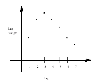
where d is the degree of the polynomial used. Models of this kind are called Almon lag models, polynomial distributed lag models, or PDLs for short. For example, Figure 19.64 shows the lag distribution that can be modeled with a low-order polynomial. Endpoint restrictions can be imposed on a PDL to require that the lag coefficients be 0 at the 0th lag, or at the final lag, or at both.

Figure 19.64: Polynomial Distributed Lags

For linear single-equation models, SAS/ETS software includes the PDLREG procedure for estimating PDL models. See Chapter 21: The PDLREG Procedure, for a more detailed discussion of polynomial distributed lags and an explanation of endpoint restrictions.

Polynomial and other distributed lag models can be estimated and simulated or forecast with PROC MODEL. For polynomial distributed lags, the %PDL macro can generate the needed programming statements automatically.

The %PDL Macro

The SAS macro %PDL generates the programming statements to compute the lag coefficients of polynomial distributed lag models and to apply them to the lags of variables or expressions.

To use the %PDL macro in a model program, you first call it to declare the lag distribution; later, you call it again to apply the PDL to a variable or expression. The first call generates a PARMS statement for the polynomial parameters and assignment statements to compute the lag coefficients. The second call generates an expression that applies the lag coefficients to the lags of the specified variable or expression. A PDL can be declared only once, but it can be used any number of times (that is, the second call can be repeated).

The initial declaratory call has the general form

%PDL ( pdlname, nlags, degree , R=code , OUTEST=dataset ) ;

where pdlname is a name (up to 32 characters) that you give to identify the PDL, nlags is the lag length, and degree is the degree of the polynomial for the distribution. The R=code is optional for endpoint restrictions. The value of code can be FIRST (for upper), LAST (for lower), or BOTH (for both upper and lower endpoints). See Chapter 21: The PDLREG Procedure, for a discussion of endpoint restrictions. The option OUTEST=dataset creates a data set that contains the estimates of the parameters and their covariance matrix.

The later calls to apply the PDL have the general form

   %PDL( pdlname, expression )

where pdlname is the name of the PDL and expression is the variable or expression to which the PDL is to be applied. The pdlname given must be the same as the name used to declare the PDL.

The following statements produce the output in Figure 19.65:

proc model data=in list;
   parms int pz;
   %pdl(xpdl,5,2);
   y = int + pz * z + %pdl(xpdl,x);
   %ar(y,2,M=ULS);
   id i;
fit y / out=model1 outresid converge=1e-6;
run;

Figure 19.65: %PDL Macro Estimates

The MODEL Procedure

Nonlinear OLS Estimates
Term	Estimate	Approx Std Err	t Value	Approx Pr > \|t\|	Label
XPDL_L0	1.568788	0.0935	16.77	<.0001	PDL(XPDL,5,2) coefficient for lag0
XPDL_L1	0.564917	0.0328	17.22	<.0001	PDL(XPDL,5,2) coefficient for lag1
XPDL_L2	-0.05063	0.0593	-0.85	0.4155	PDL(XPDL,5,2) coefficient for lag2
XPDL_L3	-0.27785	0.0517	-5.37	0.0004	PDL(XPDL,5,2) coefficient for lag3
XPDL_L4	-0.11675	0.0368	-3.17	0.0113	PDL(XPDL,5,2) coefficient for lag4
XPDL_L5	0.43267	0.1362	3.18	0.0113	PDL(XPDL,5,2) coefficient for lag5

This second example models two variables, Y1 and Y2, and uses two PDLs:

proc model data=in;
   parms int1 int2;
   %pdl( logxpdl, 5, 3 )
   %pdl( zpdl, 6, 4 )
   y1 = int1 + %pdl( logxpdl, log(x) ) + %pdl( zpdl, z );
   y2 = int2 + %pdl( zpdl, z );
   fit y1 y2;
run;

A (5,3) PDL of the log of X is used in the equation for Y1. A (6,4) PDL of Z is used in the equations for both Y1 and Y2. Since the same ZPDL is used in both equations, the lag coefficients for Z are the same for the Y1 and Y2 equations, and the polynomial parameters for ZPDL are shared by the two equations. See Example 19.5 for a complete example and comparison with PDLREG.