Suppose a rock quarry needs equipment to use the next five years. It has two alternatives:
-
a box loader and conveyer system that has a one-time cost of $264,000
-
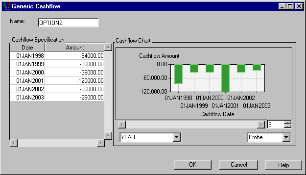
a two-shovel loader, which costs $84,000 but has a yearly operating cost of $36,000. This loader has a service life of three years, which necessitates the purchase of a new loader for the final two years of the rock quarry project. Assume the second loader also costs $84,000 and its salvage value after its two-year service is $10,000. A SAS data set that describes this is available at
SASHELP.ROCKPIT
You expect a 13% MARR. Which is the better alternative?
To create the cashflows, follow these steps:
-
Create a cashflow with the single amount –264,000. Date the amount 01JAN1998 to be consistent with the SAS data set you load.
-
Load
SASHELP.ROCKPITinto a second cashflow, as displayed in Figure 57.2.
To compute the time values of these investments, follow these steps:
-
Select both cashflows.
-
Select Analyze
 Time Value. This opens the Time Value Analysis dialog box.
-
Enter the date 01JAN1998 into the Dates area.
-
Enter 13 for the Constant MARR.
-
Click Create Time Value Summary.
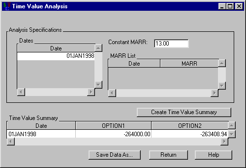
As shown in Figure 57.3, option 1 has a time value of –$264,000.00 naturally on 01JAN1998. However, option 2 has a time value of –$263,408.94, which is slightly less expensive.