Statistics of Fit
This section explains the goodness-of-fit statistics reported to measure how well different models fit the data. The statistics of fit for the various forecasting models can be viewed or stored in a data set by using the Model Viewer window.
Statistics of fit are computed by using the actual and forecasted values for observations in the period of evaluation. One-step forecasted values are used whenever possible, including the case when a hold-out sample contains no missing values. If a one-step forecast for an observation cannot be computed due to missing values for previous series observations, a multi-step forecast is computed, using the minimum number of steps as the previous nonmissing values in the data range permit.
The various statistics of fit reported are as follows. In these formulas, n is the number of nonmissing observations and k is the number of fitted parameters in the model.
-
Number of Nonmissing Observations. The number of nonmissing observations used to fit the model.
Number of Observations. The total number of observations used to fit the model, including both missing and nonmissing observations.
Number of Missing Actuals. The number of missing actual values.
Number of Missing Predicted Values. The number of missing predicted values.
Number of Model Parameters. The number of parameters fit to the data. For combined forecast, this is the number of forecast components.
Total Sum of Squares (Uncorrected). The total sum of squares for the series, SST, uncorrected for the mean:
 .
.
Total Sum of Squares (Corrected). The total sum of squares for the series, SST, corrected for the mean:
 , where
  is the series mean.
Sum of Square Errors. The sum of the squared prediction errors, SSE.
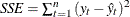 , where
  is the one-step predicted value.
Mean Squared Error. The mean squared prediction error, MSE, calculated from the one-step-ahead forecasts.
 . This formula enables you to evaluate small hold-out samples.
Root Mean Squared Error. The root mean square error (RMSE),
 .
.
Mean Absolute Percent Error. The mean absolute percent prediction error (MAPE),
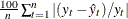 .The summation ignores observations where
  .
.
Mean Absolute Error. The mean absolute prediction error,
 .
.
R-Square. The
 statistic,
 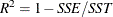 . If the model fits the series badly, the model error sum of squares, SSE, can be larger than SST and the statistic will be negative.
Adjusted R-Square. The adjusted
statistic, 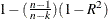 .
.
Amemiya’s Adjusted R-Square. Amemiya’s adjusted
, 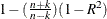 .
.
Random Walk R-Square. The random walk
statistic (Harvey’s  statistic by using the random walk model for comparison),
 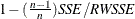 , where
  , and
, and 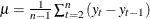 .
.
Akaike’s Information Criterion. Akaike’s information criterion (AIC),
 .
.
Schwarz Bayesian Information Criterion. Schwarz Bayesian information criterion (SBC or BIC),
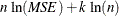 .
.
Amemiya’s Prediction Criterion. Amemiya’s prediction criterion,
 .
.
Maximum Error. The largest prediction error.
Minimum Error. The smallest prediction error.
Maximum Percent Error. The largest percent prediction error,
 . The summation ignores observations where .
Minimum Percent Error. The smallest percent prediction error,
 . The summation ignores observations where .
Mean Error. The mean prediction error,
 .
.
Mean Percent Error. The mean percent prediction error,
 . The summation ignores observations where .