PROC MODEL: Properties of the Estimates

Properties of the Estimates

All of the methods are consistent. Small sample properties might not be good for nonlinear models. The tests and standard errors reported are based on the convergence of the distribution of the estimates to a normal distribution in large samples.

These nonlinear estimation methods reduce to the corresponding linear systems regression methods if the model is linear. If this is the case, PROC MODEL produces the same estimates as PROC SYSLIN.

Except for GMM, the estimation methods assume that the equation errors for each observation are identically and independently distributed with a 0 mean vector and positive definite covariance matrix $\text{[math]}$ consistently estimated by S. For FIML, the errors need to be normally distributed. There are no other assumptions concerning the distribution of the errors for the other estimation methods.

The consistency of the parameter estimates relies on the assumption that the S matrix is a consistent estimate of $\text{[math]}$ . These standard error estimates are asymptotically valid, but for nonlinear models they might not be reliable for small samples.

The S matrix used for the calculation of the covariance of the parameter estimates is the best estimate available for the estimation method selected. For S-iterated methods, this is the most recent estimation of $\text{[math]}$ . For OLS and 2SLS, an estimate of the S matrix is computed from OLS or 2SLS residuals and used for the calculation of the covariance matrix. For a complete list of the S matrix used for the calculation of the covariance of the parameter estimates, see Table 19.1.

Missing Values

An observation is excluded from the estimation if any variable used for FIT tasks is missing, if the weight for the observation is not greater than 0 when weights are used, or if a DELETE statement is executed by the model program. Variables used for FIT tasks include the equation errors for each equation, the instruments, if any, and the derivatives of the equation errors with respect to the parameters estimated. Note that variables can become missing as a result of computational errors or calculations with missing values.

The number of usable observations can change when different parameter values are used; some parameter values can be invalid and cause execution errors for some observations. PROC MODEL keeps track of the number of usable and missing observations at each pass through the data, and if the number of missing observations counted during a pass exceeds the number that was obtained using the previous parameter vector, the pass is terminated and the new parameter vector is considered infeasible. PROC MODEL never takes a step that produces more missing observations than the current estimate does.

The values used to compute the Durbin-Watson, R $\text{[math]}$ , and other statistics of fit are from the observations used in calculating the objective function and do not include any observation for which any needed variable was missing (residuals, derivatives, and instruments).

Details on the Covariance of Equation Errors

There are several S matrices that can be involved in the various estimation methods and in forming the estimate of the covariance of parameter estimates. These S matrices are estimates of $\text{[math]}$ , the true covariance of the equation errors. Apart from the choice of instrumental or noninstrumental methods, many of the methods provided by PROC MODEL differ in the way the various S matrices are formed and used.

All of the estimation methods result in a final estimate of $\text{[math]}$ , which is included in the output if the COVS option is specified. The final S matrix of each method provides the initial S matrix for any subsequent estimation.

This estimate of the covariance of equation errors is defined as

$\text{[math]}$

where $\text{[math]}$ is composed of the equation residuals computed from the current parameter estimates in an $\text{[math]}$ matrix and D is a diagonal matrix that depends on the VARDEF= option.

For VARDEF=N, the diagonal elements of D are $\text{[math]}$ , where n is the number of nonmissing observations. For VARDEF=WGT, n is replaced with the sum of the weights. For VARDEF=WDF, n is replaced with the sum of the weights minus the model degrees of freedom. For the default VARDEF=DF, the ith diagonal element of D is $\text{[math]}$ , where df $\text{[math]}$ is the degrees of freedom (number of parameters) for the ith equation. Binkley and Nelson (1984) show the importance of using a degrees-of-freedom correction in estimating $\text{[math]}$ . Their results indicate that the DF method produces more accurate confidence intervals for N3SLS parameter estimates in the linear case than the alternative approach they tested. VARDEF=N is always used for the computation of the FIML estimates.

For the fixed S methods, the OUTSUSED= option writes the S matrix used in the estimation to a data set. This S matrix is either the estimate of the covariance of equation errors matrix from the preceding estimation, or a prior $\text{[math]}$ estimate read in from a data set when the SDATA= option is specified. For the diagonal S methods, all of the off-diagonal elements of the S matrix are set to 0 for the estimation of the parameters and for the OUTSUSED= data set, but the output data set produced by the OUTS= option contains the off-diagonal elements. For the OLS and N2SLS methods, there is no previous estimate of the covariance of equation errors matrix, and the option OUTSUSED= saves an identity matrix unless a prior $\text{[math]}$ estimate is supplied by the SDATA= option. For FIML, the OUTSUSED= data set contains the S matrix computed with VARDEF=N. The OUTS= data set contains the S matrix computed with the selected VARDEF= option. Both versions of the S matrix appear in the printed output for FIML.

If the COVS option is used, the method is not S-iterated, S is not an identity, and the OUTSUSED= matrix is included in the printed output.

For the methods that iterate the covariance of equation errors matrix, the S matrix is iteratively re-estimated from the residuals produced by the current parameter estimates. This S matrix estimate iteratively replaces the previous estimate until both the parameter estimates and the estimate of the covariance of equation errors matrix converge. The final OUTS= matrix and OUTSUSED= matrix are thus identical for the S-iterated methods.

Nested Iterations

By default, for S-iterated methods, the S matrix is held constant until the parameters converge once. Then the S matrix is reestimated. One iteration of the parameter estimation algorithm is performed, and the S matrix is again reestimated. This latter process is repeated until convergence of both the parameters and the S matrix. Since the objective of the minimization depends on the S matrix, this has the effect of chasing a moving target.

When the NESTIT option is specified, iterations are performed to convergence for the structural parameters with a fixed S matrix. The S matrix is then reestimated, the parameter iterations are repeated to convergence, and so on until both the parameters and the S matrix converge. This has the effect of fixing the objective function for the inner parameter iterations. It is more reliable, but usually more expensive, to nest the iterations.

R-Square Statistic

For unrestricted linear models with an intercept successfully estimated by OLS, R $\text{[math]}$ is always between 0 and 1. However, nonlinear models do not necessarily encompass the dependent mean as a special case and can produce negative R $\text{[math]}$ statistics. Negative R $\text{[math]}$ statistics can also be produced even for linear models when an estimation method other than OLS is used and no intercept term is in the model.

R $\text{[math]}$ is defined for normalized equations as

$\text{[math]}$

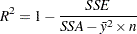where SSA is the sum of the squares of the actual $\text{[math]}$ ’s and $\text{[math]}$ are the actual means. R $\text{[math]}$ cannot be computed for models in general form because of the need for an actual Y.