| The VARMAX Procedure |
| Bayesian VAR and VARX Modeling |
Consider the VAR( ) model
 |
or
 |
When the parameter vector  has a prior multivariate normal distribution with known mean
  and covariance matrix
  , the prior density is written as
 |
The likelihood function for the Gaussian process becomes
 |
 |
 |
|||
 |
|
 |
Therefore, the posterior density is derived as
 |
where the posterior mean is
 |
and the posterior covariance matrix is
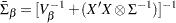 |
In practice, the prior mean and the prior variance need to be specified. If all the parameters are considered to shrink toward zero, the null prior mean should be specified. According to Litterman (1986), the prior variance can be given by
 |
where  is the prior variance of the
  th element of
  ,
,  is the prior standard deviation of the diagonal elements of ,
  is a constant in the interval
  , and
, and  is the
  th diagonal element of
  . The deterministic terms have diffused prior variance. In practice, you replace the by the diagonal element of the ML estimator of in the nonconstrained model.
For example, for a bivariate BVAR(2) model,
 |
 |
 |
|||
 |
|
 |
with the prior covariance matrix
 |
 |
 |
|||
|
|
 |
For the Bayesian estimation of integrated systems, the prior mean is set to the first lag of each variable equal to one in its own equation and all other coefficients at zero. For example, for a bivariate BVAR(2) model,
|
|
 |
|||
|
|
 |
Forecasting of BVAR Modeling
The mean squared error is used to measure forecast accuracy (Litterman 1986). The MSE of the forecast is
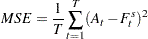 |
where  is the actual value at time
  and
and  is the forecast made
  periods earlier.
Bayesian VARX Modeling
The Bayesian vector autoregressive model with exogenous variables is called the BVARX(,) model. The form of the BVARX(,) model can be written as
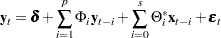 |
The parameter estimates can be obtained by representing the general form of the multivariate linear model,
|
The prior means for the AR coefficients are the same as those specified in BVAR(). The prior means for the exogenous coefficients are set to zero.
Some examples of the Bayesian VARX model are as follows:
model y1 y2 = x1 / p=1 xlag=1 prior;
   model y1 y2 = x1 / p=(1 3) xlag=1 nocurrentx
                      prior=(lambda=0.9 theta=0.1);
Copyright © SAS Institute, Inc. All Rights Reserved.