| The QLIM Procedure |
| Stochastic Frontier Production and Cost Models |
Stochastic frontier production models were first developed by Aigner, Lovell, and Schmidt (1977) and Meeusen and van den Broeck (1977). Specification of these models allow for random shocks of the production or cost but also include a term for technological or cost inefficiency. Assuming that the production function takes a log-linear Cobb-Douglas form, the stochastic frontier production model can be written as
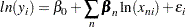 |
where  . The
. The  term represents the stochastic error component and
  is the nonnegative, technology inefficiency error component. The error component is assumed to be distributed iid normal and independently from . If
  , the error term,
  , is negatively skewed and represents technology inefficiency. If
  , the error term is positively skewed and represents cost inefficiency. PROC QLIM models the error component as a half normal, exponential, or truncated normal distribution.
The Normal-Half Normal Model
In case of the normal-half normal model, is iid  , is iid
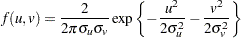
  with and independent of each other. Given the independence of error terms, the joint density of
  and
and  can be written as
 |
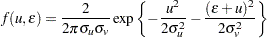
Substituting  into the preceding equation gives
 |
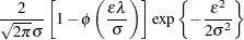
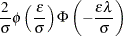
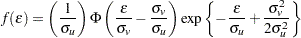
Integrating out to obtain the marginal density function of  results in the following form:
 |
 |
 |
|||
 |
|
 |
|||
|
|
 |
where  and
and  .
.
In the case of a stochastic frontier cost model,  and
and
 |
The log-likelihood function for the production model with  producers is written as
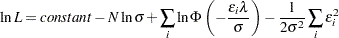 |
The Normal-Exponential Model
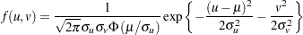
Under the normal-exponential model, is iid and is iid exponential. Given the independence of error term components and , the joint density of and can be written as
 |
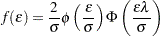
The marginal density function of for the production function is
|
|
|
|||
|
|
 |
and the marginal density function for the cost function is equal to
 |
The log-likelihood function for the normal-exponential production model with producers is
 |
The Normal-Truncated Normal Model
The normal-truncated normal model is a generalization of the normal-half normal model by allowing the mean of to differ from zero. Under the normal-truncated normal model, the error term component is iid  and is iid
  . The joint density of and can be written as
 |
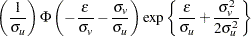
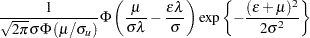
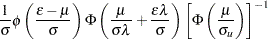
The marginal density function of for the production function is
|
|
|
|||
|
|
 |
|||
|
|
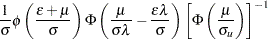 |
and the marginal density function for the cost function is
|
|
 |
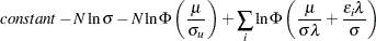
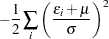
The log-likelihood function for the normal-truncated normal production model with producers is
 |
|
 |
|||
|
|
 |
For more detail on normal-half normal, normal-exponential, and normal-truncated models, see Kumbhakar and Knox Lovell (2000) and Coelli, Prasada Rao, and Battese (1998).
Copyright © SAS Institute, Inc. All Rights Reserved.