| The MODEL Procedure |
| Error Covariance Structure Specification |
One of the key assumptions of regression is that the variance of the errors is constant across observations. Correcting for heteroscedasticity improves the efficiency of the estimates.
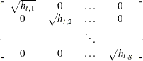
Consider the following general form for models:
 |
 |
 |
|||
 |
|
 |
|||
 |
|
 |
|||
 |
|
 |
where  .
.
For models that are homoscedastic,
 |
If you have a model that is heteroscedastic with known form, you can improve the efficiency of the estimates by performing a weighted regression. The weight variable, using this notation, would be  .
.
If the errors for a model are heteroscedastic and the functional form of the variance is known, the model for the variance can be estimated along with the regression function.
To specify a functional form for the variance, assign the function to an H.var variable where var is the equation variable. For example, if you want to estimate the scale parameter for the variance of a simple regression model
 |
you can specify
   proc model data=s;
      y = a * x + b;
      h.y = sigma**2;
   fit y;
Consider the same model with the following functional form for the variance:
 |
This would be written as
   proc model data=s;
      y = a * x + b;
      h.y = sigma**2 * x**(2*alpha);
   fit y;
There are three ways to model the variance in the MODEL procedure: feasible generalized least squares, generalized method of moments, and full information maximum likelihood.
Feasible GLS
A simple approach to estimating a variance function is to estimate the mean parameters  by using some auxiliary method, such as OLS, and then use the residuals of that estimation to estimate the parameters
  of the variance function. This scheme is called feasible GLS. It is possible to use the residuals from an auxiliary method for the purpose of estimating because in many cases the residuals consistently estimate the error terms.
For all estimation methods except GMM and FIML, using the H.var syntax specifies that feasible GLS is used in the estimation. For feasible GLS, the mean function is estimated by the usual method. The variance function is then estimated using pseudo-likelihood (PL) function of the generated residuals. The objective function for the PL estimation is
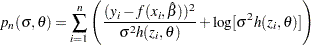 |
Once the variance function has been estimated, the mean function is reestimated by using the variance function as weights. If an S-iterated method is selected, this process is repeated until convergence (iterated feasible GLS).
Note that feasible GLS does not yield consistent estimates when one of the following is true:
The variance is unbounded.
There is too much serial dependence in the errors (the dependence does not fade with time).
There is a combination of serial dependence and lag dependent variables.
The first two cases are unusual, but the third is much more common. Whether iterated feasible GLS avoids consistency problems with the last case is an unanswered research question. For more information see Davidson and MacKinnon (1993, pp. 298–301) or Gallant (1987, pp. 124–125) and Amemiya (1985, pp. 202–203).
One limitation is that parameters cannot be shared between the mean equation and the variance equation. This implies that certain GARCH models, cross-equation restrictions of parameters, or testing of combinations of parameters in the mean and variance component are not allowed.
Generalized Method of Moments
In GMM, normally the first moment of the mean function is used in the objective function.
|
|
 |
|||
 |
|
 |
To add the second moment conditions to the estimation, add the equation
 |
to the model. For example, if you want to estimate  for linear example above, you can write
   proc model data=s;
      y = a * x + b;
      eq.two = resid.y**2 - sigma**2;
   fit y two/ gmm;
   instruments x;
   run;
This is a popular way to estimate a continuous-time interest rate processes (see Chan et al. 1992). The H.var syntax automatically generates this system of equations.
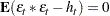
To further take advantage of the information obtained about the variance, the moment equations can be modified to
 |
|
|
|||
 |
|
|
For the above example, this can be written as
   proc model data=s;
      y = a * x + b;
      eq.two = resid.y**2 - sigma**2;
      resid.y = resid.y / sigma;
   fit y two/ gmm;
   instruments x;
   run;
Note that, if the error model is misspecified in this form of the GMM model, the parameter estimates might be inconsistent.
Full Information Maximum Likelihood
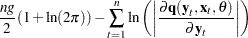
For FIML estimation of variance functions, the concentrated likelihood below is used as the objective function. That is, the mean function is coupled with the variance function and the system is solved simultaneously.
 |
|
 |
|||
 |
 |
 |
where  is the number of equations in the system.
The HESSIAN=GLS option is not available for FIML estimation that involves variance functions. The matrix used when HESSIAN=CROSS is specified is a crossproducts matrix that has been enhanced by the dual quasi-Newton approximation.
Examples
You can specify a GARCH(1,1) model as follows:
   proc model data=modloc.usd_jpy;

                /* Mean model --------*/
      jpyret = intercept ;

                /* Variance model ----------------*/
      h.jpyret = arch0
               + arch1 * xlag( resid.jpyret ** 2, mse.jpyret  )
               + garch1 * xlag(h.jpyret, mse.jpyret) ;

      bounds arch0 arch1 garch1 >= 0;

   fit jpyret / method=marquardt fiml;
   run;
Note that the BOUNDS statement is used to ensure that the parameters are positive, a requirement for GARCH models.
EGARCH models are used because there are no restrictions on the parameters. You can specify a EGARCH(1,1) model as follows:
   proc model data=sasuser.usd_dem ;

             /* Mean model ----------*/
     demret = intercept ;

                /* Variance model ----------------*/
     if ( _OBS_ =1 )  then
       h.demret = exp( earch0 + egarch1 * log(mse.demret)  );
     else
       h.demret = exp( earch0 + earch1 * zlag( g)
                            + egarch1 * log(zlag(h.demret)));
     g = - theta * nresid.demret + abs( nresid.demret ) - sqrt(2/3.1415);

   fit demret / method=marquardt fiml  maxiter=100 converge=1.0e-6;
   run;
Copyright © SAS Institute, Inc. All Rights Reserved.