In mixed logit models, an individual’s utility from any alternative can be decomposed into a deterministic component, , which is a linear combination of observed variables, and a stochastic component, ,

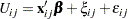where is a vector of observed variables that relate to individual and alternative , is a vector of parameters, is an error component that can be correlated among alternatives and heteroscedastic for each individual, and is a random term with zero mean that is independently and identically distributed over alternatives and individuals. The conditional logit model is derived if you assume has an iid Gumbel distribution and .

The mixed logit model assumes a general distribution for and an iid Gumbel distribution for . Denote the density function of the error component as , where is a parameter vector of the distribution of . The choice probability of alternative for individual is written as

where the conditional choice probability for a given value of is the logit

Since is not given, the unconditional choice probability, , is the integral of the conditional choice probability, , over the distribution of . This model is called "mixed logit" since the choice probability is a mixture of logits with as the mixing distribution.

In general, the mixed logit model does not have an exact likelihood function because the probability does not always have a closed form solution. Therefore, a simulation method is used for computing the approximate probability,

where is the number of simulation replications and is a simulated probability. The simulated log-likelihood function is computed as

where

For simulation purposes, assume that the error component has a specific structure,

where is a vector of observed data and is a random vector with zero mean and density function . The observed data vector () of the error component can contain some or all elements of . The component induces heteroscedasticity and correlation across unobserved utility components of the alternatives. This allows flexible substitution patterns among the alternatives. The th element of vector is distributed as

Therefore, can be specified as

where

or

In addition, is a vector of random parameters (random coefficients). Random coefficients allow heterogeneity across individuals in their sensitivity to observed exogenous variables. The observed data vector, , is a subset of . The following three types of distributions for the random coefficients are supported, where the th element of is denoted as :

• Normally distributed coefficient with the mean and spread being estimated.

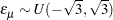
• Uniformly distributed coefficient with the mean and spread being estimated. A uniform distribution with mean and spread is .

• Lognormally distributed coefficient. The coefficient is calculated as

  where and are parameters that are estimated.

The estimate of spread for normally, uniformly, and lognormally distributed coefficients can be negative. The absolute value of the estimated spread can be interpreted as an estimate of standard deviation for normally distributed coefficients.

A detailed description of mixed logit models can be found, for example, in Brownstone and Train (1999).