| The QLIM Procedure |
| Ordinal Discrete Choice Modeling |
Binary Probit and Logit Model
The binary choice model is
 |
where value of the latent dependent variable,  , is observed only as follows:
 |
 |
 |
|||
 |
 |
 |
The disturbance,  , of the probit model has standard normal distribution with the distribution function (CDF)
 |
The disturbance of the logit model has standard logistic distribution with the CDF
 |
The binary discrete choice model has the following probability that the event  occurs:
 |
The log-likelihood function is
 |
where the CDF  is defined as
  for the probit model while
  for logit. The first order derivative of the logit model are
 |
The probit model has more complicated derivatives
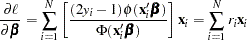 |
where
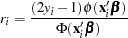 |
Note that the logit maximum likelihood estimates are  times greater than probit maximum likelihood estimates, since the probit parameter estimates,
  , are standardized, and the error term with logistic distribution has a variance of
  .
.
Ordinal Probit/Logit
When the dependent variable is observed in sequence with  categories, binary discrete choice modeling is not appropriate for data analysis. McKelvey and Zavoina (1975) proposed the ordinal (or ordered) probit model.
Consider the following regression equation:
 |
where error disturbances, , have the distribution function  . The unobserved continuous random variable,
  , is identified as categories. Suppose there are
  real numbers,
  , where
  ,
,  ,
,  , and
, and  . Define
 |
The probability that the unobserved dependent variable is contained in the  th category can be written as
 |
The log-likelihood function is
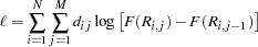 |
where
 |
The first derivatives are written as
 |
 |
where  and
and  if
if  . When the ordinal probit is estimated, it is assumed that
  . The ordinal logit model is estimated if
  . The first threshold parameter,
  , is estimated when the LIMIT1=VARYING option is specified. By default (LIMIT1=ZERO), so that
  threshold parameters (
 ) are estimated.
The ordered probit models are analyzed by Aitchison and Silvey (1957), and Cox (1970) discussed ordered response data by using the logit model. They defined the probability that belongs to th category as
 |
where and . Therefore, the ordered response model analyzed by Aitchison and Silvey can be estimated if the LIMIT1=VARYING option is specified. Note that  .
.
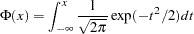
Goodness-of-Fit Measures
The goodness-of-fit measures discussed in this section apply only to discrete dependent variable models.
McFadden (1974) suggested a likelihood ratio index that is analogous to the  in the linear regression model:
 |
where  is the value of the maximum likelihood function and
  is a likelihood function when regression coefficients except an intercept term are zero. It can be shown that can be written as
 |
where  is the number of responses in category .
Estrella (1998) proposes the following requirements for a goodness-of-fit measure to be desirable in discrete choice modeling:
The measure must take values in
 , where 0 represents no fit and 1 corresponds to perfect fit.
 The measure should be directly related to the valid test statistic for significance of all slope coefficients.
The derivative of the measure with respect to the test statistic should comply with corresponding derivatives in a linear regression.
Estrella’s (1998) measure is written
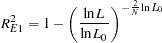 |
An alternative measure suggested by Estrella (1998) is
 |
where  is computed with null slope parameter values,
  is the number observations used, and
  represents the number of estimated parameters.
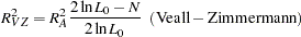
Other goodness-of-fit measures are summarized as follows:
 |
 |
 |
 |
 |
where  and
and  .
.
Copyright © 2008 by SAS Institute Inc., Cary, NC, USA. All rights reserved.