For an example on dynamic panel estimation using GMM option, see The Cigarette Sales Data: Dynamic Panel Estimation with GMM.

Consider the case of the following general model:

The variables can include ones that are correlated or uncorrelated to the individual effects, predetermined, or strictly exogenous. The and are cross-sectional and time series fixed effects, respectively. Arellano and Bond (1991) show that it is possible to define conditions that should result in a consistent estimator.

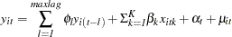
Consider the simple case of an autoregression in a panel setting (with only individual effects):

Differencing the preceding relationship results in:

where .

Obviously, is not exogenous. However, Arellano and Bond (1991) show that it is still useful as an instrument, if properly lagged.

For (assuming the first observation corresponds to time period 1) you have,

Using as an instrument is not a good idea since . Therefore, since it is not possible to form a moment restriction, you discard this observation.

For you have,

Clearly, you have every reason to suspect that . This condition forms one restriction.

For , both 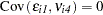and 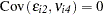must hold.

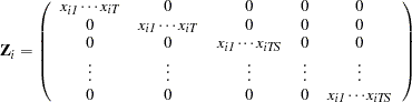
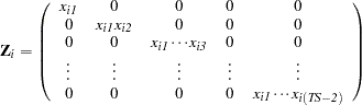
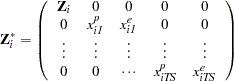
Proceeding in that fashion, you have the following matrix of instruments,

Using the instrument matrix, you form the weighting matrix as

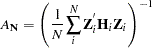The initial weighting matrix is

Note that the maximum size of the matrix is T–2. The origins of the initial weighting matrix are the expected error covariances. Notice that on the diagonals,

and off diagonals,

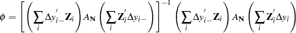
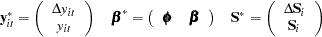
If you let the vector of lagged differences (in the series ) be denoted as and the dependent variable as , then the optimal GMM estimator is

Using the estimate, , you can obtain estimates of the errors, , or the differences, . From the errors, the variance is calculated as,

where is the total number of observations.

Furthermore, you can calculate the variance of the parameter as,

Alternatively, you can view the initial estimate of the as a first step. That is, by using , you can improve the estimate of the weight matrix, .

Instead of imposing the structure of the weighting, you form the matrix through the following:

You then complete the calculation as previously shown. The PROC PANEL option TWOSTEP specifies this estimation.

The case of multiple right-hand-side variables illustrates more clearly the power of Arellano and Bond (1991) and Arellano and Bover (1995).

Considering the general case you have:

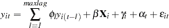It is clear that lags of the dependent variable are both not exogenous and correlated to the fixed effects. However, the independent variables can fall into one of several categories. An independent variable can be correlated and exogenous, uncorrelated and exogenous, correlated and predetermined, and uncorrelated and predetermined. The category in which an independent variable is found influences when or whether it becomes a suitable instrument. Note, however, that neither PROC PANEL nor Arellano and Bond require that a regressor be an instrument or that an instrument be a regressor.

First, consider the question of exogenous or endogenous. An exogenous variable is not correlated with the error term in the model at all. Therefore, all observations (on the exogenous variable) become valid instruments at all time periods. If the model has only one instrument and it happens to be exogenous, then the optimal instrument matrix looks like,

The situation for the predetermined variables becomes a little more difficult. A predetermined variable is one whose future realizations can be correlated to current shocks in the dependent variable. With such an understanding, it is admissible to allow all current and lagged realizations as instruments. In other words you have,

When the data contain a mix of endogenous, exogenous, and predetermined variables, the instrument matrix is formed by combining the three. The third observation would have one observation on the dependent variable as an instrument, three observations on the predetermined variables as instruments, and all observations on the exogenous variables.

There is yet another set of moment restrictions that can be employed. An uncorrelated variable means that the variable’s level is not affected by the individual specific effect. You write the general model presented above as:

where .

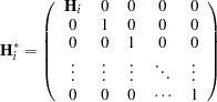
Since the variables are uncorrelated with and uncorrelated with the error, you can perform a system estimation with the difference and level equations. That is, the uncorrelated variables imply moment restrictions on the level equation. If you denote the new instrument matrix with the full complement of instruments available by a and both and are uncorrelated, then you have:

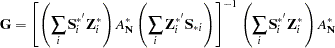
The formation of the initial weighting matrix becomes somewhat problematic. If you denote the new weighting matrix with a , then you can write the following:

where

To finish, you write out the two equations (or two stages) that are estimated.

where is the matrix of all explanatory variables, lagged endogenous, exogenous, and predetermined.

Let be given by

Using the information above,

If the TWOSTEP or ITGMM option is not requested, estimation terminates here. If it terminates, you can obtain the following information.

Variance of the error term comes from the second stage equation—that is,

where is the number of regressors.

The variance covariance matrix can be obtained from

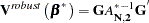
Alternatively, a robust estimate of the variance covariance matrix can be obtained by specifying the ROBUST option. Without further reestimation of the model, the matrix is recalculated as follows:

And the weighting matrix becomes

Using the information above, you construct the robust variance covariance matrix from the following:

Let denote a temporary matrix.

The robust variance covariance estimate of is:

Alternatively, the new weighting matrix can be used to form an updated estimate of the regression parameters. This results when the TWOSTEP option is requested. In short,

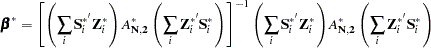The variance covariance estimate of the two step becomes

As a final note, it possible to iterate more than twice by specifying the ITGMM option. Such a multiple iteration should result in a more stable estimate of the variance covariance estimate. PROC PANEL allows two convergence criteria. Convergence can occur in the parameter estimates or in the weighting matrices. Iterate until

or

where ATOL is the tolerance for convergence in the weighting matrix and BTOL is the tolerance for convergence in the parameter estimate matrix. The default convergence criteria is BTOL = 1E–8 for PROC PANEL.