| The PANEL Procedure |
| The One-Way Random-Effects Model |
The specification for the one-way random-effects model is
 |
Let  ),
),  , and
, and  , with
  and
and  . Define
  and
and  .
.
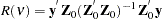
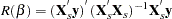
In the one-way model, estimation proceeds in a two-step fashion. First, you obtain estimates of the variance of the  and
and  . There are multiple ways to derive these estimates; PROC PANEL provides four options. All four options are valid for balanced or unbalanced panels. Once these estimates are in hand, they are used to form a weighting factor
  , and estimation proceeds via OLS on partial deviations from group means.
PROC PANEL gives the following options for variance component estimators.
Fuller and Battese’s Method
The Fuller and Battese method for estimating variance components can be obtained with the option VCOMP = FB and the option RANONE. The variance components are given by the following equations (see Baltagi and Chang (1994) and Fuller and Battese (1974) for the approach in the two-way model). Let
 |
 |
 |
 |
The estimator of the error variance is given by
 |
If the NOINT option is specified, the estimator is
 |
The estimator of the cross-sectional variance component is given by
 |
Note that the error variance is the variance of the residual of the within estimator.
According to Baltagi and Chang (1994), the Fuller and Battese method is appropriate to apply to both balanced and unbalanced data. The Fuller and Battese method is the default for estimation of one-way random-effects models with balanced panels. However, the Fuller and Battese method does not always obtain nonnegative estimates for the cross section (or group) variance. In the case of a negative estimate, a warning is printed and the estimate is set to zero.
Wansbeek and Kapteyn’s Method
The Wansbeek and Kapteyn method for estimating variance components can be obtained by setting VCOMP = WK (together with the option RANONE). The estimation of the one-way unbalanced data model is performed by using a specialization (Baltagi and Chang 1994) of the approach used by Wansbeek and Kapteyn (1989) for unbalanced two-way models. The Wansbeek and Kapteyn method is the default for unbalanced data. If just RANONE is specified, without the VCOMP= option, PROC PANEL estimates the variance component under Wansbeek and Kapteyn’s method.
The estimation of the variance components is performed by using a quadratic unbiased estimation (QUE) method. This involves focusing on quadratic forms of the centered residuals, equating their expected values to the realized quadratic forms, and solving for the variance components.
Let
 |
 |
where the residuals  are given by
  if there is an intercept and by
 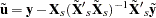 if there is not.
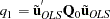
Consider the expected values
 |
 |
 |
where  and
and  are obtained by equating the quadratic forms to their expected values.
The estimator of the error variance is the residual variance of the within estimate. The Wansbeek and Kapteyn method can also generate negative variance components estimates.
Wallace and Hussain’s Method
The Wallace and Hussain method for estimating variance components can be obtained by setting VCOMP = WH (together with the option RANONE). Wallace-Hussain estimates start from OLS residuals on a data that are assumed to exhibit groupwise heteroscedasticity. As in the Wansbeek and Kapteyn method, you start with
 |
 |
However, instead of using the 'true' errors, you substitute the OLS residuals. You solve the system
 |
 |
The constants  are given by
 |
 |
 |
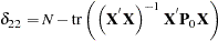 |
where tr() is the trace operator on a square matrix.
Solving this system produces the variance components. This method is applicable to balanced and unbalanced panels. However, there is no guarantee of positive variance components. Any negative values are fixed equal to zero.
Nerlove’s Method
The Nerlove method for estimating variance components can be obtained by setting VCOMP = NL. The Nerlove method (see Baltagi 1995, page 17) is assured to give estimates of the variance components that are always positive. Furthermore, it is simple in contrast to the previous estimators.
If  is the
  th fixed effect, Nerlove’s method uses the variance of the fixed effects as the estimate of . You have
 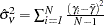 , where
  is the mean fixed effect. The estimate of
  is simply the residual sum of squares of the one-way fixed-effects regression divided by the number of observations.
With the variance components in hand, from any method, the next task is to estimate the regression model of interest. For each individual, you form a weight ( ) as follows:
 |
 |
where  is the th cross section’s time observations.
Taking the , you form the partial deviations,
 |
 |
where  and
and  are cross section means of the dependent variable and independent variables (including the constant if any), respectively.
The random-effects  is then the result of simple OLS on the transformed data.
Copyright © 2008 by SAS Institute Inc., Cary, NC, USA. All rights reserved.