Decisions
Each modeling node can
make a decision for each case in a scoring data set, based on numerical
consequences specified via a decision matrix and cost variables or
cost constants. The decision matrix can specify profit, loss, or revenue.
In the GUI, the decision matrix is provided via the Target Profile.
With a previously scored data set containing posterior probabilities,
decisions can also be made using PROC DECIDE, which reads the decision
matrix from a decision data set.
When you use decision
processing, the modeling nodes compute summary statistics giving the
total and average profit or loss for each model. These profit and
loss summary statistics are useful for selecting models. To use these
summary statistics for model selection, you must specify numeric consequences
for making each decision for each value of the target variable. It
is your responsibility to provide reasonable numbers for the decision
consequences based on your particular application.
In some applications,
the numeric consequences of each decision might not all be known at
the time you are training the model. Hence, you might want to perform
what-if analyses to explore the effects of different decision consequences
using the Model Comparison node. In particular, when one of the decisions
is to "do nothing," the profit charts in the Model Comparison
node provide a convenient way to see the effect of applying different
thresholds for the do-nothing decision.
To use profit charts,
the do-nothing decision should not be included in the decision matrix;
the Model Comparison node will implicitly supply a do-nothing decision
when computing the profit charts. When you omit the do-nothing decision
from the profit matrix so you can obtain profit charts, you should
not use the profit and loss summary statistics for comparing models,
since these summary statistics will not incorporate the implicit do-nothing
decision. This topic is discussed further in Decision Thresholds and
Profit Charts.
The decision matrix
contains columns (decision variables) corresponding to each decision,
and rows (observations) corresponding to target values. The values
of the decision variables represent target-specific consequences,
which might be profit, loss, or revenue. These consequences are the
same for all cases being scored. A decision data set might contain
prior probabilities in addition to the decision matrix.
For a categorical target
variable, there should be one row for each class. The value in the
decision matrix located at a given row and column specifies the consequence
of making the decision corresponding to the column when the target
value corresponds to the row. The decision matrix is allowed to contain
rows for classes that do not appear in the data being analyzed. For
a profit or revenue matrix, the decision is chosen to maximize the
expected profit. For a loss matrix, the decision is chosen to minimize
the expected loss.
For an interval target
variable, each row defines a knot in a piecewise linear spline function.
The consequence of making a decision is computed by linear interpolation
in the corresponding column of the decision matrix. If the predicted
target value is outside the range of knots in the decision matrix,
the consequence of a decision is computed by linear extrapolation.
Decisions are made to maximize the predicted profit or minimize the
predicted loss.
For each decision, there
might also be either a cost variable or a numeric cost constant. The
values of cost variables represent case-specific consequences, which
are always treated as costs. These consequences do not depend on the
target values of the cases being scored. Costs are used for computing
return on investment as (revenue-cost)/cost.
Cost variables can be
specified only if the decision matrix contains revenue, not profit
or loss. Hence, if revenues and costs are specified, profits are computed
as revenue minus cost. If revenues are specified without costs, the
costs are assumed to be zero. The interpretation of consequences as
profits, losses, revenues, and costs is needed only to compute return
on investment. You can specify values in the decision matrix that
are target-specific consequences but that might have some practical
interpretation other than profit, loss, or revenue. Likewise, you
can specify values for the cost variables that are case-specific consequences
but that might have some practical interpretation other than costs.
If the revenue/ cost interpretation is not applicable, the values
computed for return on investment might not be meaningful. There are
some restrictions on the use of cost variables in the Decision
Tree node; see the documentation on the Decision Tree node for more
information.
In principle, consequences
need not be the sum of target-specific and case-specific terms, but
SAS Enterprise Miner does not support such nonadditive consequences.
For a categorical target
variable, you can use a decision matrix to classify cases by specifying
the same number of decisions as classes and having each decision correspond
to one class. However, there is no requirement for the number of decisions
to equal the number of classes except for ordinal target variables
in the Decision Tree node.
For example, suppose
there are three classes designated red, blue, and green. For an identity
decision matrix, the average profit is equal to the correct-classification
rate:
|
Target Value:
|
Decision:
|
||
|---|---|---|---|
|
Red
|
Blue
|
Green
|
|
|
Red
|
1
|
0
|
0
|
|
Blue
|
0
|
1
|
0
|
|
Green
|
0
|
0
|
1
|
To obtain the misclassification
rate, you can specify a loss matrix with zeros on the diagonal and
ones everywhere else:
|
Target Value:
|
Decision:
|
||
|---|---|---|---|
|
Red
|
Blue
|
Green
|
|
|
Red
|
0
|
1
|
1
|
|
Blue
|
1
|
0
|
1
|
|
Green
|
1
|
1
|
0
|
If it is 20 times more
important to classify red cases correctly than blue or green cases,
you can specify a diagonal profit matrix with a profit of 20 for classifying
red cases correctly and a profit of one for classifying blue or green
cases correctly:
|
Target Value:
|
Decision:
|
||
|---|---|---|---|
|
Red
|
Blue
|
Green
|
|
|
Red
|
20
|
0
|
0
|
|
Blue
|
0
|
1
|
0
|
|
Green
|
0
|
0
|
1
|
When you use a diagonal
profit matrix, the decisions depend only on the products of the prior
probabilities and the corresponding profits, not on their separate
values. Hence, for any given combination of priors and diagonal profit
matrix, you can make any change to the priors (other than replacing
a zero with a nonzero value) and find a corresponding change to the
diagonal profit matrix that leaves the decisions unchanged, even though
the expected profit for each case might change.
Similarly, for any given
combination of priors and diagonal profit matrix, you can find a set
of priors that will yield the same decisions when used with an identity
profit matrix. Therefore, using a diagonal profit matrix does not
provide you with any power in decision making that could not be achieved
with no profit matrix by choosing appropriate priors (although the
profit matrix might provide an advantage in interpretability). Furthermore,
any two by two decision matrix can be transformed into a diagonal
profit matrix as discussed in the following section on Decision Thresholds
and Profit Charts.
When the decision matrix
is three by three or larger, it might not be possible to diagonalize
the profit matrix, and some nondiagonal profit matrices will produce
effects that could not be achieved by manipulating the priors. To
show the effect of a nondiagonalizable decision matrix, the data in
the upper left plot of the following figure were generated to have
three classes, shown as red circles, blue crosses, and green triangles.
Each class has 100 training
cases with a bivariate normal distribution. The training data were
used to fit a linear logistic regression model using the Neural Network
engine. The posterior probabilities are shown in the upper right plot.
Classification according to the posterior probabilities yields linear
classification boundaries as shown in the lower left plot. Use of
a nondiagonalizable decision matrix causes the decision boundaries
in the lower right plot to be rotated in comparison with the classification
boundaries, and the decision boundaries are curved rather than linear.
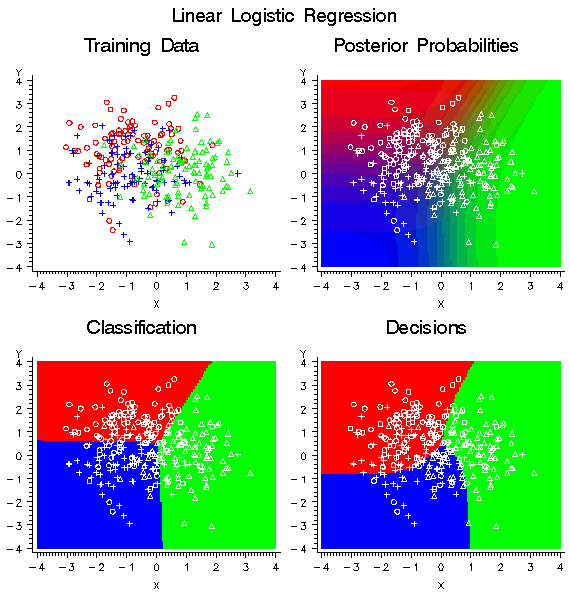
The decision matrix
that produced the curved decision boundaries is shown in the following
table:
In each row, the two
profit values for misclassification are different. Hence, it is impossible
to diagonalize the matrix by adding a constant to each row. Consider
the blue row. The greatest profit is for a correct assignment into
blue, but there is also a smaller but still substantial profit for
assignment into red. There is no profit for assigning red into blue,
so the red-blue decision boundary is moved toward the blue mean in
comparison with the classification boundary based on posterior probabilities.
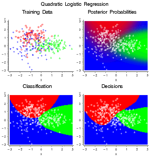
The following figure shows the effect of the same nondiagonal profit
matrix on a quadratic logistic regression model.
For the Neural Network
and Regression nodes, a separate decision is made for each case. For
the Decision Tree node, a common decision is made for all cases in
the same leaf of the tree, so when different cases have different
costs, the average cost in the leaf is used in place of the individual
costs for each case. That is, the profit equals the revenue minus
the average cost among all training cases in the same leaf. Hence,
a single decision is assigned to all cases in the same leaf of a tree.
The decision alternative
assigned to a validation, test, or scoring case ignores any cost associated
with the case. The new data are assumed similar to the training data
in cost as well as predictive relations. However, the actual cost
values for each case are used for the investment cost, ROI, and quantities
that depend on the actual target value.
Decision and cost matrices
do not affect:
-
Estimating parameters in the Regression node
-
Learning weights in the Neural Network node
-
Growing (as opposed to pruning) trees in the Decision Tree node unless the target is ordinal
-
Residuals, which are based on posteriors before adjustment for priors
-
Error functions such as deviance or likelihood
-
Fit statistics such as MSE based on residuals or error functions
-
Posterior probabilities
-
Classification
-
Misclassification rate.
-
Growing trees in the Decision Tree node when the target is ordinal
-
Decisions
-
Expected profit or loss
-
Profit and loss summary statistics, including the relative contribution of each class.
Decision and cost matrices
will by default affect the following processes if and only if there
are two or more decisions:
-
Choice of models in the Regression node
-
Early stopping in the Neural Network node
-
Pruning trees in the Decision Tree node.
Formulas will be presented
first for the Neural Network and Regression nodes. Let:
t
be an index for target
values (classes)
d
be an index for decisions
i
be an index for cases
nd
be the number of decisions
Class(t)
be the set of indices
of cases belonging to target t
Profit(t,d)
be the profit for
making decision d when the target is t
Loss(t,d)
be the loss for making
decision d when the target is t
Revenue(t,d)
be the revenue for
making decision d when the target is t
Cost(i,d)
be the cost for making
decision d for case i
Q(i,t,d)
be the combined consequences
for making decision d when the target is t for case i
Prior(t)
be the prior probability
for target t
Paw(t)
be the prior-adjustment
weight for target t
Post(i,t)
be the posterior probability
of target t for case i
F(i)
be the frequency for
case i
T(i)
be the index of the
actual target value for case i
A(i,d)
be the expected profit
of decision d for case i
B(i)
be the best possible
profit for case i based on the actual target value
C(i)
be the computed profit
for case i based on the actual target value
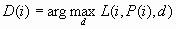
D(i)
be the index of the
decision chosen by the model for case i
E(i)
be the expected profit
for case i of the decision chosen by the model
IC(i)
be the investment cost
for case i for the decision chosen by the model
ROI(i)
be the return on investment
for case i for the decision chosen by the model.
These quantities are
related by the following formulas:
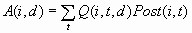
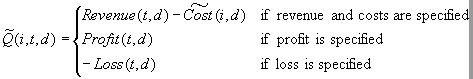
When the target variable
is categorical, the expected profit for decision d in case i is:
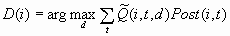
For each case i, the
decision is made by choosing D(i) to be the value of d that maximizes
the expected profit:

If two or more decisions
are tied for maximum expected profit, the first decision in the user-specified
list of decisions is chosen.
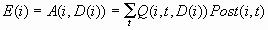
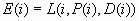
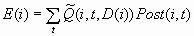
The expected profit
E(i) is the expected combined consequence for the chosen decision
D(i), computed as a weighted average over the target values of the
combined consequences, using the posterior probabilities as weights:
The expected loss is
the negative of expected profit.
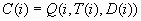
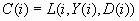
Note that E(i) and D(i)
can be computed without knowing the target index T(i). When T(i) is
known, two more quantities useful for evaluating the model can also
be computed. C(i) is the profit computed from the target value using
the decision chosen by the model:
The loss computed from
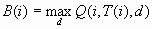
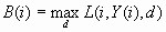
the target value is the negative of C(i). C(i) is the most important
variable for assessing and comparing models. The best possible profit
for any of the decisions, which is an upper bound for C(i), is:
The best possible loss
is the negative of B(i).
When revenue and cost
are specified, investment cost is:
And return on investment
is:
![ROI = [C(i)/IC(i)] if IC(i) > 0, = I(infinity) if IC(i) <= 0 and C(i) > 0, = (missing) if IC(i) <= 0 and C(i) = 0, = M (-infinity) if IC(i) <= 0 and C(i) < 0.](images/prede97.png)
For an interval target
variable, let:
Y(i)
be the actual target
value for case i
P(i)
be the predicted target
value for case i
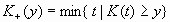
K(t)
be the knot value for
the row of the decision matrix.
For interval targets,
the predicted value is assumed to be accurate enough that no integration
over the predictive distribution is required. Define the functions:
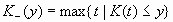
![L(i,y,d) = Q(i,K_(y),d) + [(y – K_(y))/(K+ (y) – K_(y))][Q(i,K+ (y),d) – Q(i,K_(y),d)]](images/prede100.png)
Then the decision is
made by maximizing the expected profit:
The expected profit
for the chosen decision is:
When Y(i) is known,
the profit computed from the target value using the decision chosen
by the model is:
And the best possible
profit for any of the decisions is:
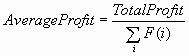
For both categorical
and interval targets, the summary statistics for decision processing
with profit and revenue matrices are computed by summation over cases
with nonmissing cost values. If no adjustment for prior probabilities
is used, the sums are weighted only by the case frequencies. Hence,
total profit and average profit are given by the following formulas:

![Average Profit = [Total Profit/Sum(i)F(i)]](images/prede106.png)
For loss matrices, total
loss and average loss are the negatives of total profit and average
profit, respectively.
If total and average
profit are adjusted for prior probabilities, an additional weight
Paw(t)is used:
![Paw(t) = [[(Prior(t))/Sum(i element of Class(t))F(i)]Sum(i)F(i)]](images/prede107.png)
Total and average profit
are then given by:
![Total Profit = Sum(i)F(i)C(i)Paw[T(i)] = Sum(i)Paw(t) Sum(i element of Class(t))F(i)C(i)](images/prede108.png)
If any class with a
positive prior probability has a total frequency of zero, total and
average profit and loss cannot be computed and are assigned missing
values. Note that the adjustment of total and average profit and loss
is done only if you explicitly specify prior probabilities; the adjustment
is not done when the implicit priors based on the training set proportions
are used.
The adjustment for prior
probabilities is not done for fit statistics such as SSE, deviance,
likelihood, or misclassification rate. For example, consider the situation
shown in the following table:
|
Proportion
In
|
Unconditional
Misclassification Rate
|
|||||
|---|---|---|---|---|---|---|
|
Class
|
Operational
Data
|
Training
Data
|
Prior Probability
|
Conditional
Misclassification Rate
|
Unadjusted
|
Adjusted
|
|
Rare
|
0.1
|
0.5
|
0.1
|
0.8
|
0.5 * 0.8 + 0.5 * 0.2
= 0.50
|
0.1 * 0.8 + 0.9 * 0.2
= 0.26
|
|
Common
|
0.9
|
0.5
|
0.9
|
0.2
|
||
There is a rare class
comprising 10% of the operational data, and a common class comprising
90%. For reasons discussed in the section below on Detecting
Rare Classes, you might want to train using a balanced sample with
50% from each class. To obtain correct posterior probabilities and
decisions, you specify prior probabilities of .1 and .9 that are equal
to the operational proportions of the two classes.
Suppose the conditional
misclassification rate for the common class is low, just 20%, but
the conditional misclassification rate for the rare class is high,
80%. If it is important to detect the rare class accurately, these
misclassification rates are poor.
The unconditional misclassification
rate computed using the training proportions without adjustment for
priors is a mediocre 50%. But adjusting for priors, the unconditional
misclassification rate is apparently much better at only 26%. Hence,
the adjusted misclassification rate is misleading.
For the Decision Tree
node, the following modifications to the formulas are required. Let
Leaf(i) be the set of indices of cases in the same leaf as case i.
Then:
![Cost(i,d) = [(Sum(j element of Leaf(i)) F(j)Cost(j,d)) / (Sum(J element of Leaf(i)) F(j))]](images/prede110.png)
The combined consequences
are:
For a categorical target,
the decision is:
And the expected profit
is:
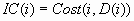
For an interval target:
![L(i,t,d) = Q(i,K_(y),d) + [(y – K_(y))/(K+ (y) – K_(y))][Q(i,K_(y),d)]](images/prede114.png)
The decision is:
![D(i) = [(arg max(d) Sum(j element of Leaf(i)) F(j)L(j, P(j), d))/(Sum(j element of Leaf(i)) F(j))]](images/prede115.png)
And the expected profit
is:
![D(i) = [(arg max(d) Sum(j element of Leaf(i)) F(j)L(j, P(j), D(i))/(Sum(j element of Leaf(i)) F(j))]](images/prede116.png)
The other formulas are
unchanged.
Copyright © SAS Institute Inc. All rights reserved.