Generalization

The critical issue in predictive modeling is generalization: how well will the model make predictions for cases that are not in the training set? Data mining models, like other flexible nonlinear estimation methods such as kernel regression, can suffer from either underfitting or overfitting (or as statisticians usually say, oversmoothing or undersmoothing). A model that is not sufficiently complex can fail to detect fully the signal in a complicated data set, leading to underfitting. A model that is too complex might fit the noise, not just the signal, leading to overfitting. Overfitting can happen even with noise-free data and, especially in neural nets, can yield predictions that are far beyond the range of the target values in the training data.

By making a model sufficiently complex, you can always fit the training data perfectly. For example, if you have N training cases and you fit a linear regression with N-1 inputs, you can always get zero error (assuming that the inputs are not singular). Even if the N-1 inputs are random numbers that are totally unrelated to the target variable, you will still get zero error on the training set. However, the predictions are worthless for such a regression model for new cases that are not in the training set.

Even if you use only one continuous input variable, by including enough polynomial terms in a regression, you can get zero training error. Similarly, you can always get a perfect fit with only one input variable by growing a tree large enough or by adding enough hidden units to a neural net.

On the other hand, if you omit an important input variable from a model, both the training error and the generalization error will be poor. If you use too few terms in a regression, or too few hidden units in a neural net, or too small a tree, then again the training error and the generalization error might be poor.

Hence, with all types of data mining models, you must strike a balance between a model that is too simple and one that is too complex. It is usually necessary to try a variety of models and then choose a model that is likely to generalize well.

There are many ways to choose a model. Some popular methods are heuristic, such as stepwise regression or CHAID tree modeling, where the model is modified in a sequence of steps that terminates when no further steps satisfy a statistical significance criterion. Such heuristic methods might be of use for developing explanatory models, but they do not directly address the question of which model will generalize best. The obvious way to approach this question directly is to estimate the generalization error of each model, and then choose the model with the smallest estimated generalization error.

There are many ways to estimate generalization error, but it is especially important not to use the training error as an estimate of generalization error. As previously mentioned, the training error can be very low even when the generalization error is very high. Choosing a model based on training error will cause the most complex model to be chosen even if it generalizes poorly.

A better way to estimate generalization error is to adjust the training error for the complexity of the model. In linear least squares regression, this adjustment is fairly simple if the input variables are assumed fixed or multivariate normal. Let

Then the average squared error for the training set is SSE/N, which is designated as ASE by SAS Enterprise Miner modeling nodes. Statistical software often reports the mean squared error, MSE=SSE/(N-P).

MSE adjusts the training error for the complexity of the model by subtracting P in the denominator, which makes MSE larger than ASE. But MSE is not a good estimate of the generalization error of the trained model. Under the usual statistical assumptions, MSE is an unbiased estimate of the generalization error of the model with the best possible ("true") weights, not the weights that were obtained by training.

Hence, a stronger adjustment is required to estimate generalization error of the trained model. One way to provide a stronger adjustment is to use Akaike's Final Prediction Error (FPE):

The formula for FPE multiplies MSE by (N+P)/N, so FPE is larger than MSE. If the input variables are fixed rather than random, FPE is an unbiased estimate of the generalization error of the trained model. If inputs and target are multivariate normal, a further adjustment is required:

This is slightly larger than FPE but has no conventional acronym.

The formulas for MSE and FPE were derived for linear least squares regression. For nonlinear models and for other training criteria, MSE and FPE are not unbiased. MSE and FPE might provide adequate approximations if the model is not too nonlinear and the number of training cases is much larger than the number of estimated weights. But simulation studies have shown, especially for neural networks, that FPE is not a good criterion for model choice, since it does not provide a sufficiently severe penalty for overfitting.

There are other methods for adjusting the training error for the complexity of the model. Two of the most popular criteria for model choice are Schwarz's Bayesian criterion, (SBC), also called the Bayesian information criterion, (BIC), and Rissanen's minimum description length principle (MDL). Although these two criteria were derived from different theoretical frameworks — SBC from Bayesian statistics and MDL from information theory — they are essentially the same. In SAS Enterprise Miner, only the acronym SBC is used. For least squares training,

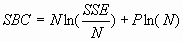
For maximum likelihood training,

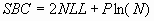
where NLL is the negative log likelihood. Smaller values of SBC are better, since smaller values of SSE or NLL are better. SBC often takes negative values. SBC is valid for nonlinear models under the usual statistical regularity conditions. Simulation studies have found that SBC works much better than FPE for model choice in neural networks.

However, the usual statistical regularity conditions might not hold for neural networks, so SBC might not be entirely satisfactory. In tree-based models, there is no well-defined number of weights, P, in the model, so SBC is not directly applicable. And other types of models and training methods exist for which no single-sample statistics such as SBC are known to be good criteria for model choice. Furthermore, none of these adjustments for model complexity can be applied to decision processing to maximize total profit. Fortunately, there are other methods for estimating generalization error and total profit that are very broadly applicable; these methods include split-sample or holdout validation, cross validation, and bootstrapping.

Split-sample validation is applicable with any type of model and any training method. You split the available data into a training set and a validation set, usually by simple random sampling or stratified random sampling. You train the model using only the training set. You estimate the generalization error for each model that you train by scoring the validation set. Then you select the model with the smallest validation error. Split-sample validation is fast and is often the method of choice for large data sets. For small data sets, split-sample validation is not so useful because it does not make efficient use of the data.

For small data sets, cross validation is generally preferred to split-sample validation. Cross validation works by splitting the data several ways, training a different model for each split, and then combining the validation results across all the splits. In k-fold cross validation, you divide the data into k subsets of (approximately) equal size. You train the model k times, each time leaving out one of the subsets from training, but using only the omitted subset to compute the error criterion. If k equals the sample size, this is called "leave-one-out" cross validation.

"Leave-v-out" is a more elaborate and expensive version of cross validation that involves leaving out all possible subsets of v cases. Cross validation makes efficient use of the data because every case is used for both training and validation. But, of course, cross validation requires more computer time than split-sample validation. SAS Enterprise Miner provides leave-one-out cross validation in the Regression node; k-fold cross validation can be done easily with SAS macros.

In the literature of artificial intelligence and machine learning, the term "cross validation" is often applied incorrectly to split-sample validation, causing much confusion. The distinction between cross validation and split-sample validation is extremely important because cross validation can be markedly superior for small data sets. On the other hand, leave-one-out cross validation might perform poorly for discontinuous error functions such as the number of misclassified cases, or for discontinuous modeling methods such as stepwise regression or tree-based models. In such discontinuous situations, split-sample validation or k-fold cross validation (usually with k equal to five or ten) are preferred, depending on the size of the data set.

Bootstrapping seems to work better than cross validation in many situations, such as stepwise regression, at the cost of even more computation. In the simplest form of bootstrapping, instead of repeatedly analyzing subsets of the data, you repeatedly analyze subsamples of the data. Each subsample is a random sample with replacement from the full sample. Depending on what you want to do, anywhere from 200 to 2000 subsamples might be used. There are many more sophisticated bootstrap methods that can be used not only for estimating generalization error but also for estimating bias, standard errors, and confidence bounds.

Not all bootstrapping methods use resampling from the data — you can also resample from a nonparametric density estimate, or resample from a parametric density estimate, or, in some situations, you can use analytical results. However, bootstrapping does not work well for some methods such as tree-based models, where bootstrap generalization estimates can be excessively optimistic.

There has been relatively little research on bootstrapping neural networks. SAS macros for bootstrap inference can be obtained from Technical Support.

When numerous models are compared according to their estimated generalization error (for example, the error on a validation set), and the model with the lowest estimated generalization error is chosen for operational use, the estimate of the generalization error of the selected model will be optimistic. This optimism is a consequence of the statistical principle of regression to the mean. Each estimate of generalization error is subject to random fluctuations. Some models by chance will have an excessively high estimate of generalization error, but others will have an excessively low estimate of generalization error.

The model that wins the competition for lowest generalization error is more likely to be among the models that by chance have an excessively low estimate of generalization error. Even if the method for estimating the generalization error of each model individually provides an unbiased estimate, the estimate for the winning model will be biased downward. Hence, if you want an unbiased estimate of the generalization error of the winning model, further computations are required to obtain such an estimate.

For large data sets, the most practical way to obtain an unbiased estimate of the generalization error of the winning model is to divide the data set into three parts, not just two: the training set, the validation set, and the test set. The training set is used to train each model. The validation set is used to choose one of the models. The test data set is used to obtain an unbiased estimate of the generalization error of the chosen model.

The training/validation/test data set approach is explained by Bishop (1995, p. 372) as follows:

"Since our goal is to find the network having the best performance on new data, the simplest approach to the comparison of different networks is to evaluate the error function using data that is independent of that used for training. Various networks are trained by minimization of an appropriate error function defined with respect to a training data set. The performance of the networks is then compared by evaluating the error function using an independent validation set, and the network having the smallest error with respect to the validation set is selected. This approach is called the hold out method. Since this procedure can itself lead to some overfitting to the validation set, the performance of the selected network should be confirmed by measuring its performance on a third independent set of data called a test set."