Multivariate Techniques

Principal Components Analysis

The purpose of principal component analysis is to derive a small number of independent linear combinations (principal components) of a set of variables that retain as much of the information in the original variables as possible.

For example, suppose you are interested in examining the relationship among measures of food consumption from different sources. The sample data set Protein records the amount of protein consumed from nine food groups for each of 25 European countries. The nine food groups are red meat (RedMt), white meat (WhiteMt), eggs (Eggs), milk (Milk), fish (Fish), cereal (Cereal), starch (Starch), nuts (Nuts), and fruits and vegetables (FruVeg).

Open the Protein Data Set

The data are provided in the Analyst Sample Library. To access this Analyst sample data set, follow these steps:

Select Tools Sample Data ...
Select Protein.
Click OK to create the sample data set in your Sasuser directory.
Select File Open By SAS Name ...
Select Sasuser from the list of Libraries.
Select Protein from the list of members.
Click OK to bring the Protein data set into the data table.

Request the Principal Components Analysis

To perform a principal components analysis, follow these steps:

Select Statistics Multivariate Principal Components ...
Highlight all of the quantitative variables (RedMt, WhiteMt, Eggs, Milk, Fish, Cereal, Starch, Nuts, and FruVeg).
Click on the Variables button.

The goal of this analysis is to determine the principal components of all protein sources. Therefore, all of the protein source variables are included in the Variables list, as displayed in Figure 13.2. The character variable Country is an identifier variable and is omitted from the Variables list.

Note that you can analyze a partial correlation or covariance matrix by specifying the variables to be partialed out in the Partial list. The full correlation matrix is used for this analysis.

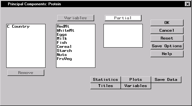Figure 13.2: Principal Components Dialog

The default principal components analysis includes simple statistics, the correlation matrix for the analysis variables, and the associated eigenvalues and eigenvectors.

Request Principal Component Plots

You can use the Plots dialog to request a scree plot or component plots. A scree plot is useful in determining the appropriate number of components to interpret. It displays the eigenvalues on the vertical axis and the principal component number on the horizontal axis.

To request a scree plot, follow these steps:

Click on the Plots button in the main dialog.
Select Create scree plot.

Figure 13.3 displays the Scree Plot tab, in which a scree plot of the positive eigenvalues is requested.

Figure 13.3: Principal Components: Plots Dialog,Scree Plot Tab

A component plot displays the component score of each observation for a pair of components. When you specify an Id variable, the values of that variable are also displayed in the plot.

To request a component plot in addition to the scree plot, follow these steps.

Click on the Component Plot tab in the Plots dialog.
Select Create component plots.
Click on the down arrow in the box labeled Type:
Select Enhanced. An enhanced component plot displays the variable names and values of the Id variable in the plot.
Select the variable Country in the Id variable list.
Click on the Id button to select the variable Country as an Id variable.

You can also enter the Dimensions for which you want plots. For example, to request plots of the first versus second, first versus third, and second versus third principal components, you type the values 1 and 3.

Click OK.

Figure 13.4 displays the Component Plot tab, which requests an enhanced component plot.

Figure 13.4: Principal Components: Plots Dialog,Component Plot Tab

Click OK in the Principal Components dialog to perform the analysis.

Review the Results

Figure 13.5 displays simple statistics and correlations among the variables.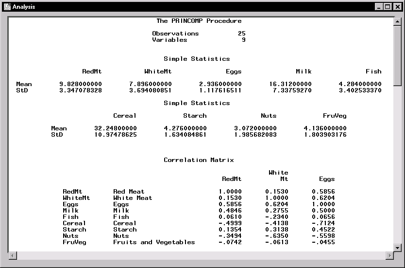

Figure 13.5: Principal Components: Simple Statistics and Correlations

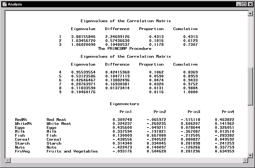Figure 13.6: Principal Components: Eigenvectors and Eigenvalues

Figure 13.6 displays the eigenvalues and eigenvectors of the correlation matrix for the nine variables. The eigenvalues indicate that four components provide a reasonable summary of the data, accounting for about 84% of the total variance. Subsequent components each contribute 5% or less.

The table of eigenvectors in Figure 13.6 reveals that the first eigenvector has equally large loadings on all of the animal-protein variables. This suggests that the first component is primarily a measure of animal-protein consumption. This eigenvector also has a large loading on the variable Starch and negative loadings on the variables Cereal and Nuts.

The second eigenvector has high positive loadings on the variables Fish, Starch, and FruVeg. This component seems to account for diets in coastal regions or warmer climates. The remaining components are not as easily identified.

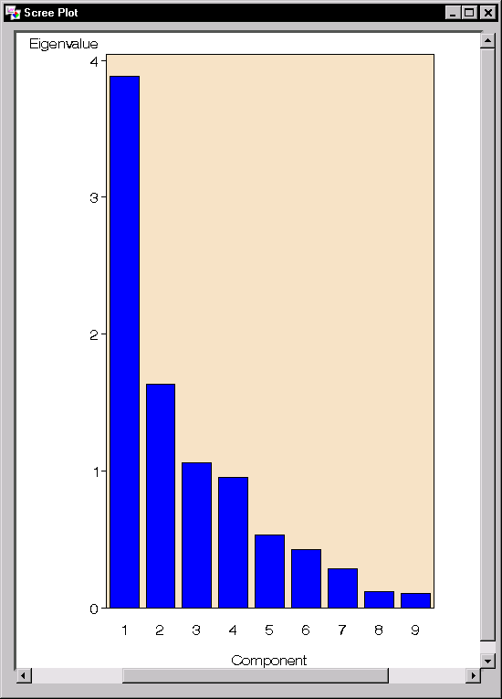Figure 13.7: Principal Components: Scree Plot

The scree plot displayed in Figure 13.7 shows a gradual decrease in eigenvalues. However, the contributions are relatively low after the fourth component, which agrees with the preceding conclusion that four principal components provide a reasonable summary of the data.

The following enhanced component plot (Figure 13.8) displays the relationship between the first two components; each observation is identified by country.

In addition, the plot is enhanced to depict the correlations between the variables and the components. This correlation is often called the component loading. The amount by which each variable "loads" on a component is measured by its correlation with the component.

In Figure 13.8, each vector corresponds to one of the analysis variables and is proportional to its component loading. For example, the variables Eggs, Milk, and RedMt all load heavily on the first component. The variables Fish and FruVeg load heavily on the second component but load very little on the first component.

The information provided by the variable Country reveals that western European countries tend to consume protein from more expensive sources (that is, meat, eggs, and milk), while countries near the Mediterranean Sea rely more heavily on fruits, vegetables, nuts, and fish for their protein sources. Eastern European countries rely more on cereal crops and nuts to supply their protein.

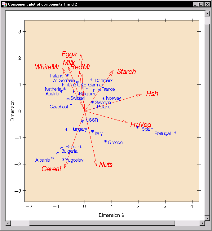Figure 13.8: Principal Components: Scores and Component Loading Plot

Top of Page