Regression

Logistic Regression

Logistic regression enables you to investigate the relationship between a categorical outcome and a set of explanatory variables. The outcome, or response, can be dichotomous (yes, no) or ordinal (low, medium, high). When you have a dichotomous response, you are performing standard logistic regression. When you are modeling an ordinal response, you are fitting a proportional odds model.

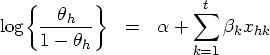
You can express the logistic model for describing the variation among probabilities $\{\theta_{h} \}$ as

$\theta_{h} & = & \{1 + \exp [- \alpha - \sum_{k=1}^t {\beta}_{k} x_{hk} ] \}^{-1}$

where $\alpha$ is the intercept parameter, ${{{{{\beta}}}}}$ is a vector of t regression parameters, and x'_h is a row vector of explanatory variables corresponding to the hth subpopulation.

You can show that the odds of success for the hth group are

$\frac {\theta_{h}} {1-\theta_{h}} & = \exp \{\alpha + \sum_{k=1}^t\beta_k x_{hk} \}$

By taking logs on both sides, you obtain a linear model for the logit:

$\log \biggl \{ \frac {\theta_{h}} {1-\theta_{h}} \biggr \} & = & \alpha + \sum_{k=1}^t {\beta}_{k} x_{hk}$

This is the log odds of success to failure for the hth subpopulation. A nice property of the logistic model is that all possible values of $(\alpha + {{x}^'_{h} {{{{{\beta}}}}})$ in $(-\infty,\infty)$ map into (0,1) for $\theta_{h}$ . Note that $\exp\{\beta_{k}\}$ are the odds ratios. Maximum likelihood methods are used to estimate $\alpha$ and ${{{{{\beta}}}}}.$

In a study on the presence of coronary artery disease, walk-in patients at a clinic were examined for symptoms of coronary artery disease. Investigators also administered an ECG. Interest lies in determining whether there is a relationship between presence or absence of coronary artery disease and ECG score and gender of patient. Logistic regression is the appropriate tool for such an investigation.

The data set analyzed in this example is called Coronary2. It contains the following variables:

sex: sex (m or f)
ecg: ST segment depression (low, medium, or high)
age: patient age
ca: disease (yes or no)

The task includes performing a logistic analysis to determine an appropriate model.

Open the Coronary2 Data Set

The data are provided in the Analyst Sample Library. To open the Coronary2 data set, follow these steps:

Select Tools Sample Data ...
Select Coronary2.
Click OK to create the sample data set in your Sasuser directory.
Select File Open By SAS Name ...
Select Sasuser from the list of Libraries.
Select Coronary2 from the list of members.
Click OK to bring the Coronary2 data set into the data table.

Request the Logistic Regression Analysis

To request the logistic regression analysis, follow these steps:

Select Statistics Regression Logistic ...
Ensure that Single trial is selected as the Dependent type.
Select ca from the candidate list as the dependent variable.
Select ecg and sex from the candidate list as the class variables.
Select age from the candidate list as the quantitative variable.
Select yes from the drop-down list for Model Pr{ }:

Note that Model Pr{ }: determines which value of the dependent variable the model is based on; usually, the value representing an event (such as yes or success) is chosen.

Figure 11.13 displays the resulting dialog.

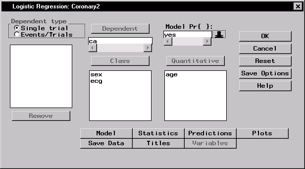Figure 11.13: Logistic Regression Dialog

Specify the Model

By default, a main effects model is fit. To define a different model, with terms such as interactions, or to specify various model selection methods, such as forward selection or backward elimination, use the Model dialog.

To specify a forward selection model with main effects and their interactions, follow these steps:

Click on the Model button in the main dialog.
Highlight the variables age, ecg, and sex in the Explanatory: list of the model dialog.
Click on the Factorial button to specify main effects and their interactions.

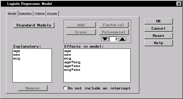Figure 11.14: Logistic Regression: Model Dialog,Model Tab

Figure 11.14 displays the Model dialog with the terms age, ecg, sex, and their interactions selected as effects in the model.

Note that you can build specific models with the Add, Cross, and Factorial buttons, or you can select a model by clicking on the Standard Models button and making a selection from the pop-up list. From this list, you can request that your model include main effects only or effects up to two-way interactions.

Now, to specify your model-building technique, follow these steps:

Click on the Selection tab.
Select Forward selection. The forward selection technique starts with a default model and adds significant variables to the model according to the specified criteria.
To specify which variables to include in every model, click on the Include tab, and select the variables age, ecg, and sex.
Click OK.

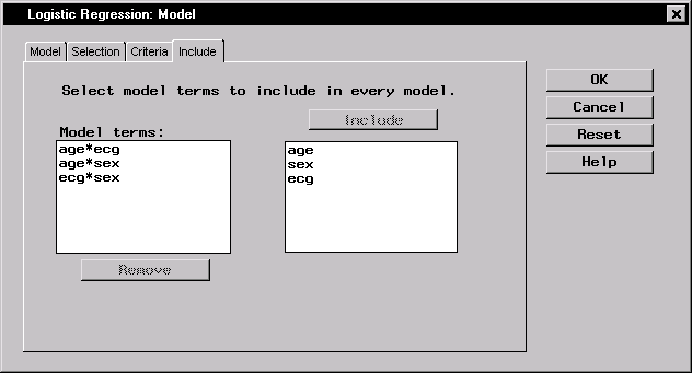Figure 11.15: Logistic Regression: Model Dialog,Include Tab

Figure 11.15 displays the Include tab with the terms age, ecg, and sex selected as model terms to be included in every model.

When you have completed your selections, click OK in the main dialog to produce your analysis.

Review the Results

Figure 11.16 displays the "Testing Global Null Hypothesis: BETA = 0" table, which lists statistics that test whether the parameters are collectively equal to zero. This is similar to the overall F statistic in a regression model.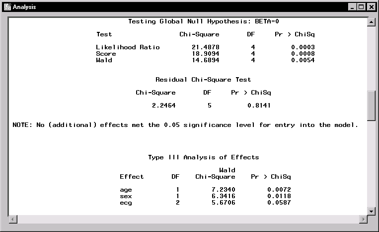

Figure 11.16: Logistic Regression: Analysis Results

When the explanatory variables in a logistic regression are relatively small in number and are qualitative, you can request a goodness-of-fit test. However, when you also have quantitative variables, the sample size requirements for these tests are not met. An alternative strategy for testing goodness of fit in this case is to examine the residual score statistic. This criterion is based on the relationship of the residuals of the model with other potential explanatory variables. If an association exists, then the additional explanatory variable should also be included in the model. This test is distributed as chi-square, with degrees of freedom equal to the difference in the number of parameters in the original model and the number of parameters in the expanded model.

The residual score statistic is displayed in Figure 11.16 as the "Residual Chi-Square Test" table. Since the difference in the number of parameters for the expanded model and the original model is 9 - 4 = 5, the score statistic has 5 degrees of freedom. Since the value of the statistic is 2.24 and the p-value is 0.81, the main effects model fits adequately and no additional interactions need to be added.

The "Type III Tests of Effects" table provides Wald chi-square statistics that indicate that both age and sex are clearly significant at the $\alpha = 0.05$ level of significance. The ecg variable approaches significance, with the Wald statistic of 5.67 and p = 0.059. Although you may want to delete the ecg variable because it does not meet the $\alpha = 0.05$ significance criteria, there may be reasons for keeping it.

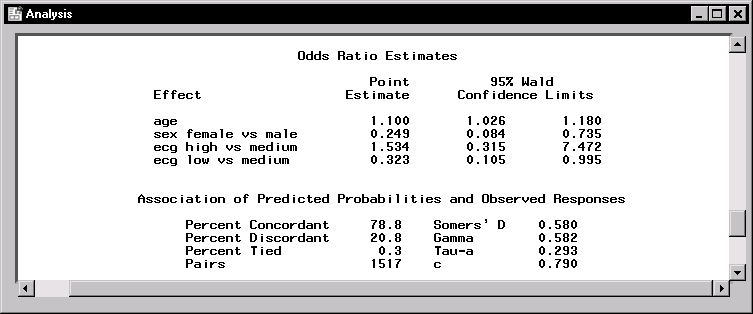Figure 11.17: Logistic Regression: Analysis Results

Figure 11.17 displays odds ratio estimates and statistics describing the association of predicted probabilities and observed responses. The value of 1.10 for age is the extent to which the odds of coronary heart disease increase each year. The odds ratio for sex, 0.249, is the odds for females relative to males adjusted for age and ecg. Thus, the odds of coronary heart diseases for females are approximately one-fourth that of males.

Top of Page